
I have proposed an experiment to test the ideas discussed in the previous pages. The details of my proposed experiment can be found in these papers: 2015, 2024, or in this preprint. An earlier version of the experiment can be found in this preprint (published in 2008), and a simplified summary or a “proof of concept” can be found in this preprint (published in 2015).
The central goal of the proposed experiment is to test the hypothesis that quantum correlations are a consequence of—or a measure of—the torsion 

![\displaystyle \leqslant\sqrt{\,\lim_{\,n\,\gg\,1}\left[\,\frac{1}{n}\sum_{k\,=\,1}^{n}\, \big\{\,4\,+\,4\,{\cal T}_{\,{\bf a\,a'}}({\lambda}^k)\,{\cal T}_{\,{\bf b'\,b}}({\lambda}^k)\,\big\}\,\right]} \ \ \ \ \](https://s0.wp.com/latex.php?latex=%5Cdisplaystyle+%5Cleqslant%5Csqrt%7B%5C%2C%5Clim_%7B%5C%2Cn%5C%2C%5Cgg%5C%2C1%7D%5Cleft%5B%5C%2C%5Cfrac%7B1%7D%7Bn%7D%5Csum_%7Bk%5C%2C%3D%5C%2C1%7D%5E%7Bn%7D%5C%2C+%5Cbig%5C%7B%5C%2C4%5C%2C%2B%5C%2C4%5C%2C%7B%5Ccal+T%7D_%7B%5C%2C%7B%5Cbf+a%5C%2Ca%27%7D%7D%28%7B%5Clambda%7D%5Ek%29%5C%2C%7B%5Ccal+T%7D_%7B%5C%2C%7B%5Cbf+b%27%5C%2Cb%7D%7D%28%7B%5Clambda%7D%5Ek%29%5C%2C%5Cbig%5C%7D%5C%2C%5Cright%5D%7D+%5C+%5C+%5C+%5C+%5C+&bg=ffffff&fg=000000&s=0&c=20201002)


This upper bound is derived in the last appendix of this paper (see also this paper). The experiment can be performed either in the outer space or in a terrestrial laboratory. In the latter case the effects of gravity and air resistance would complicate matters, but it may be possible to choose experimental parameters carefully enough to compensate for such effects.
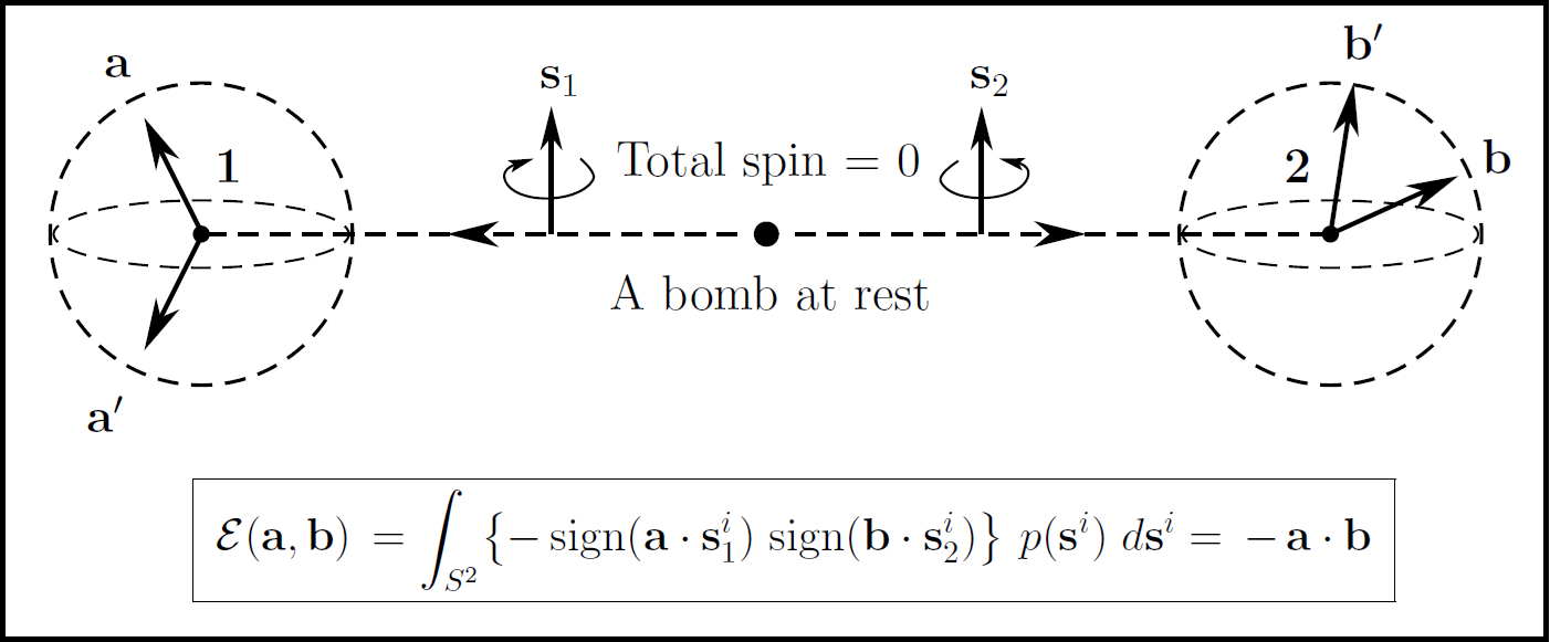
With this assumption, consider a “bomb” made out of a hollow toy ball of diameter, say, three centimeters. The thin hemispherical shells of uniform density that make up the ball are snapped together at their rims in such a manner that a slight increase in temperature would pop the ball open into its two constituents with considerable force. A small lump of density much greater than the density of the ball is attached on the inner surface of each shell at a random location, so that, when the ball pops open, not only would the two shells propagate with equal and opposite linear momenta orthogonal to their common plane, but would also rotate with equal and opposite spin momenta about a random axis in space. The volume of the attached lumps can be as small as a cubic millimeter, whereas their mass can be comparable to the mass of the ball. This will facilitate some 
Now consider a large ensemble of such balls, identical in every respect except for the relative locations of the two lumps (affixed randomly on the inner surface of each shell). The balls are then placed over a heater—one at a time—at the center of the experimental setup, with the common plane of their shells held perpendicular to the horizontal direction of the setup. Although initially at rest, a slight increase in temperature of each ball will eventually eject its two shells towards the observation stations, situated at a chosen distance in the mutually opposite directions. Instead of selecting the directions 


Once the actual directions of the angular momenta for a large ensemble of shells on both sides are fully recorded, the two computers are instructed to randomly choose a pair of reference directions, say 


![\displaystyle {\cal E}({\bf a},\,{\bf b})\,=\lim_{\,n\,\gg\,1}\!\left[\frac{1}{n}\!\sum_{k\,=\,1}^{n} \{{sign}\,(+{\bf s}^k\cdot{\bf a})\}\, \{{sign}\,(-{\bf s}^k\cdot{\bf b})\}\right] \ \ \ \ \ \ \ (2)](https://s0.wp.com/latex.php?latex=%5Cdisplaystyle+%7B%5Ccal+E%7D%28%7B%5Cbf+a%7D%2C%5C%2C%7B%5Cbf+b%7D%29%5C%2C%3D%5Clim_%7B%5C%2Cn%5C%2C%5Cgg%5C%2C1%7D%5C%21%5Cleft%5B%5Cfrac%7B1%7D%7Bn%7D%5C%21%5Csum_%7Bk%5C%2C%3D%5C%2C1%7D%5E%7Bn%7D+%5C%7B%7Bsign%7D%5C%2C%28%2B%7B%5Cbf+s%7D%5Ek%5Ccdot%7B%5Cbf+a%7D%29%5C%7D%5C%2C+%5C%7B%7Bsign%7D%5C%2C%28-%7B%5Cbf+s%7D%5Ek%5Ccdot%7B%5Cbf+b%7D%29%5C%7D%5Cright%5D+%5C+%5C+%5C+%5C+%5C+%5C+%5C+%282%29&bg=ffffff&fg=000000&s=0&c=20201002)
with
![\displaystyle \lim_{\,n\,\gg\,1}\!\left[\frac{1}{n}\!\sum_{k\,=\,1}^{n} \{{sign}\,(+{\bf s}^k\cdot{\bf a})\}\right]=\,0\,=\lim_{\,n\,\gg\,1}\!\left[\frac{1}{n}\!\sum_{k\,=\,1}^{n} \{{sign}\,(-{\bf s}^k\cdot{\bf b})\}\right]\!, \ \ \ \ \ \ \ (3)](https://s0.wp.com/latex.php?latex=%5Cdisplaystyle+%5Clim_%7B%5C%2Cn%5C%2C%5Cgg%5C%2C1%7D%5C%21%5Cleft%5B%5Cfrac%7B1%7D%7Bn%7D%5C%21%5Csum_%7Bk%5C%2C%3D%5C%2C1%7D%5E%7Bn%7D+%5C%7B%7Bsign%7D%5C%2C%28%2B%7B%5Cbf+s%7D%5Ek%5Ccdot%7B%5Cbf+a%7D%29%5C%7D%5Cright%5D%3D%5C%2C0%5C%2C%3D%5Clim_%7B%5C%2Cn%5C%2C%5Cgg%5C%2C1%7D%5C%21%5Cleft%5B%5Cfrac%7B1%7D%7Bn%7D%5C%21%5Csum_%7Bk%5C%2C%3D%5C%2C1%7D%5E%7Bn%7D+%5C%7B%7Bsign%7D%5C%2C%28-%7B%5Cbf+s%7D%5Ek%5Ccdot%7B%5Cbf+b%7D%29%5C%7D%5Cright%5D%5C%21%2C+%5C+%5C+%5C+%5C+%5C+%5C+%5C+%283%29&bg=ffffff&fg=000000&s=0&c=20201002)
where n is the number of experiments performed. According to Bell’s reasoning [which amounts to setting 

where 

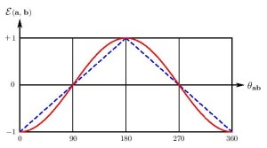
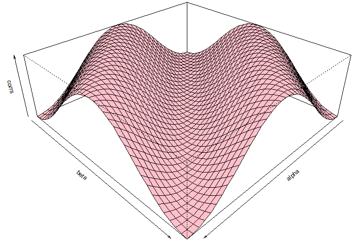
The plot below shows the difference between the correlations predicted by functions (4) and (5):
Undoubtedly, there would be many different sources of errors in a macroscopic experiment of this nature. However, at least according to David Wineland the proposed experiment is “doable.”
PS: I have recently won the 10,000 Euros offered by Richard Gill for theoretically producing the 2n angular momentum vectors, 
PPS: In the above experiment I have used two hemispheres of an “exploding” ball as a convenient means to illustrate the physical scenario. But in practice a spherically asymmetric hemisphere would wobble violently because of all sorts of inertial effects. A much better system would be something like two flexible squashy balls, squeezed together initially, and then released as if they were parts of a single bomb. This will retain the spherical symmetry of the two constituents after the “explosion” and reduce the inertial effects to near zero. For this system, however, it may be harder to maintain the singlet nature of the composite system (i.e., to maintain the vanishing total spin angular momentum of the composite system).
PPPS: In the published version of the paper the following two paragraphs have been added: 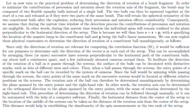
PPPPS: With the bomb made out of two squashy balls (instead of a single ball) which rapidly reshape to perfectly round spheres, the determination of spin directions would be easier, since the spin and rotation axes for each sphere would then be the same. It would still be important to eliminate aerodynamic effects before the final shapes are stabilized. A good quality check of the setup would be to compare how accurately the spins are anti-parallel, thus making sure that the singlet property for each pair of the measured spins is maintained.


Hi Joy,
Wow! Very nice blog space here! 🙂 I am not sure if I told you this before but I thought of another possibly doable macroscopic experiment. It is fairly simple thought-wise so here we go. You should be able to have someone do an experiment similar to Weihs, et al but instead of trying to count single photons, you would count a macroscopic bunch of identical in phase photons say like 10K of them. With proper filtering techniques, I think this experiment could probably be done. If the measured correlations exceed the CHSH inequality then you have macroscopic validation that Bell was wrong since the “bunches” of photons are really just a special macroscopic EM pulse.
Now, you might be asking how do we figure out what the E field value might be for 10K photons or how do we know when we have about 10K photons? I have derived a simple equation to figure that out in CGS units.
Where n = 10K identical in phase photons and lambda = 700nm wavelength. Well, perhaps we don’t need as many as 10K photons but that value for the E field strength is what we would be looking for at the detector for 10K. Of course it would be reduced by the filters, etc. but that should be able to be determined.
Perhaps you might want to run this scenario by Gregor Weihs and see if he thinks it could be done? Please ask if any questions.
Best,
Fred
Hi Fred,
Thank you for your interesting proposal. Let me see if I understand your idea correctly. We begin by preparing a sufficiently large number of “identical in phase” photons so that they can be characterized by the same initial state. It is important for the photons to be in the same initial state, because what we are looking for is correlations between the values of the E-field strength that are determined by the same initial state. Assuming that this can be done (which is a very big assumption), how do we then observe coincidences between such values? As we know, in the experiment by Weihs et al. they observed coincidences between polarizations of a single pair of photons. Detections of remote polarizations were said by them to be “coincident” if they occurred within a given time window. Are you saying that in your proposal we should look for such coincidences between the values of the E-field strength? I think that would be a very difficult thing to observe, even if we ignored the inevitable smearing in the values because of the time window. It seems to me that strong correlations would be simply averaged out because of the smearing.
On the theoretical side, it is not clear to me how such values in the E-field strength would depend on the torsion within the 3-sphere. According to my model if torsion does not play a significant role in the experiment then there will be no violation of Bell inequality.
So there is much to think about in your proposal. But it is an interesting idea nevertheless.
Best,
Joy
Hi Joy,
I am assuming that the parametric down conversion of the laser would take care of the initial state problem. Of course a stronger laser may be required. Then some kind of filter on each beam to make sure we have mostly identical inphase photons in each beam. The detectors would be detecting a certain E field value level. IOW, referring to the Weihs, et al, experiment, a detection would be a + 1 if the E field value was high enough, and -1 if low enough or zero. The polarization filters that are randomly rotated are either going to be blocking the signal or not, basically. So if this scenario can beat the CHSH inequality on coincidences, then you will have some validation that Bell was wrong. Of course the devil is in the actual details of trying to perform this experiment. 🙂
For the timing thing, the laser would have to be pulsed somehow so that we have EM pulses hitting the down convertor. And I suppose that timing need be taken into consideration of lining up the detections. But these “special” EM pulses are going to be macroscopic spinors so the torsion of the 3-sphere topology should apply I would think. I suppose only an experiment will tell though.
Best,
Fred
Hi Fred,
I understand the experiment better now.
Suppose we do the experiment and observe violations of the CHSH inequality. Would the diehard believers in non-locality be convinced by the experiment? I bet they would say: This is no surprise. The experiment only confirms Bell’s theorem, because the E field generated by the large number of photons can be easily described by QED. It is therefore no surprise that CHSH inequality is violated.
I am of course being a devil’s advocate, but how would you answer such a charge?
Put differently, how can you be sure that the “special” EM pulses are macroscopic spinors?
Best,
Joy
Hi Joy,
Of course the diehards would want to claim that the experiment is still “quantum” somehow. But we are not detecting single photons; we are detecting a macroscopic EM signal. If it beats CHSH, then that would be good enough for me of a macroscopic test and hopefully a bunch of others that aren’t diehards. I doubt if diehard Bell believers will ever change their position. As we have well seen these past years. Even if your mechanical experimental test beat Bell, they still wouldn’t accept it. But hopefully reasonable people would.
Best,
Fred
Hi Fred,
Yes, it would be good enough for me too.
There is, however, an advantage in the mechanical experiment. There is no way to fit quantum entanglement into it. The exploding bomb is obviously in a product state, not in an entangled state. I think most physicist would then accept that strong correlations are not exclusive to quantum entanglement.
Best,
Joy
Hi Joy,
A correction on my equation above; that should be E_o for the electric field and plugged into the wave equation of course.
That is true what you say about the mechanical experiment. It actually does two things.
Best,
Fred
Hi Joy,
What I wrote above does not work because there will be a racemic mix of spin 1 and -1 photons coming from the laser in each EM pulse. So a different way has to be devised to get the identical photon bunches in the two beams.
Best,
Fred
Hi Joy,
Thought about this some more. It is clear that for a macroscopic EM test, we have to simulate the singlet state somehow. Which shouldn’t be too hard to accomplish since if one beam to detector A is + 1 spin then the other to detector B has to be -1 spin and the other way around. The experiment would have to have two synchronized lasers with some kind of filters that would produce +1 spin in one beam and -1 spin in the other. Then a random optical switching device to provide the filtered EM pulses to the detector paths. I think this works as a thought experiment but perhaps a clever experimenter some day could make it a reality.
Best,
Fred
Hi Fred,
Thanks for your further thoughts. I will ask one of my friends about your proposal. He is a well known laser expert. I might be able to persuade him to read your comments.
Best,
Joy
Hi Fred, Joy,
Fred I haven’t had time to study all of your comments, but I have recently been working hard to better understand how Maxwell’s theory and Quantum theory come together best. I’m glad you’re actively thinking along those lines too. I’m not sure I understand exactly what you’re proposing, but it seems that you’re saying “the detectors would be detecting a certain E field value level (or E field strength).” I’ve spent the last few days reading Harry Paul’s “Intro to Quantum Optics”, and he states on page 41: “…it is impossible – due to the enormously high frequency of light — to measure the electric field strength.” What is detected is the energy transfer (~E^2) from the radiation field to the atomic receiver. Again, p. 21, “the electric field strength is not directly observable in the optical domain.” What is observable is the intensity. You can think of this like probability amplitude and probability. Remember that what the detectors are doing is being excited to new energy levels (or ionized) and that’s all! You may be suggesting that the E-field can be inferred, I’m not sure.
Paul’s book is a very good one (written by an experimentalist, who says: “The ‘photons of a theoretician’, as we might call them, are not at all the same thing as those described by an experimentalist who reports that a photon was absorbed at a particular position by a detector.” He is obviously very good on describing experiments, but also good on both classical and quantum optics. I recommend it.
By the way, Jonathan Dickau started a thread on FQXi about some work of Steven Kenneth Kauffmann on self-gravitational upper bounds on localized energy. In looking thru his papers (on arXiv and viXra) I found that he has some fascinating ideas, so I’m recommending his work to those who appreciate (good) new ideas.
Ed
Hi Edwin,
Yes, the electric field strength would be inferred from the square of the field strength = energy density. I mainly just presented my E_o equation above that I derived so that we have some idea about the number of identical inphase photons involved in the signal. Really, the detectors are going to either detect a signal or not detect a signal depending on the alignment of the random positions of the polarizers, etc. With 10K identical photons at 700nm wavelength, we have about 0.05 joules/cm^3 energy density. That seems high so maybe we don’t need that many photons. Probably 1K photons would do it and still is plenty macroscopic enough. I wonder what power for a laser that would require?
I will look into the book you mention above. It is obvious for sure that there is a difference between theoretical photons and experimental photons after reading a few optical experiment papers. 🙂
Yes, I made a note on Jonathan’s FQXi thread about Christoph Schiller’s work on maximum force. Kauffmann seems to have rediscovered what Schiller presented a few yeares ago and perhaps went a bit further with it. Schiller’s derivation of Einstein’s field equation (GR) starting from the concept of maximum force is pretty remarkable though.
Best,
Fred
An experiment with classical optical field has been done, and published in an optics journal: https://www.osapublishing.org/optica/abstract.cfm?URI=optica-2-7-611
It seems to be similar to the type of experiment Fred has been suggesting above.
Joy, I’ve been in talks with an electrical engineer. This made me think of your proposed experiment. What if instead of two hemispherical squishy balls, launched by some kind of temperature differential, we used two metal balls?
The idea is that we can use capacitors to instantly charge both metal balls, and the resulting coulomb force would eject them in opposite directions. The advantage is that current is much easier to control than temperature and that metal balls are less prone to get disturbed by air friction.
The only thing that is not clear to me is whether the inner lumps in the balls need to be random, but symmetric. I’d say that this needs to be the case since we want the spins to be anticorrelated.
For the metal balls, it would be rather easy to just 3D print them. We could record the data on high speed cameras (I’d say this is by far the hardest part, depending on the resolution we need). Although, the actual data processing I’d leave to you since I’m not an expert with code.
Let me know if this would be a good idea.
Btw, with another friend of mine we wrote a video for YouTube on your ideas. As soon as the first part is ready (in a few weeks at best), we are going to post it to private and show it to you if we have your permission. This first part focuses primarily on the history of EPR, von Neumann, and finally Bell’s theorem, and then we bring down the theorem itself using your analisys. Of course there is going to be your name in it and due credit to the papers. And of course we’re looking forward to any criticism if we misunderstood anything, if you have the time.
Hi Sandra,
Good thoughts. The experiment I have proposed is likely difficult to perform regardless of what material we use for balls. The idea of metal balls you suggest is good, but it also has a downside. I would imagine that metal balls would be heavier than plastic balls, so it would be more difficult to compensate for the Earth’s gravity and maintain straight trajectories. However, in addition to the advantages of using metal balls you mention, they would also be less wobbly and thus less subject to large inertial effects like precession and nutation.
The lumps inside the inner shell of the balls must be random, otherwise, we would introduce some systematic bias in the correlations between their angular momenta. The anti-correlation between them would be automatically maintained if initially they are stationary.
The idea of a YouTube video sounds good. I would be happy to review it for you and give my comments before you make it available publicly.
Joy, the video is almost done (much earlier than we thought). Probably around this weekend we’ll upload it. It’s quite long (1:20 min because of the more historic part, but the relevant part about dismantling bells theorem is around 25 minutes for now.
We wanted to introduce a bit of topology to ease the transition in a future part 2 about the 3-sphere model. One question that came up to my mind, before finalizing the video, is this: the fundamental non-linearity of the additivity of expectation values seems to be connected to the curved nature of the manifold. Parallel transported vectors on s2 take up a phase as they move around the surface, proportional to the area enclosed (holonomy). The 3-sphere is locally the Cartesian product of S1xS2, with S2 being the base space and S1 the fiber. But the global topology (important when considering different points on base space S2) is twisted, resulting in linking and relative “rotations” of the fibers. Is this twist resulting from the curvature of the base space S2, just like for parallel transported vectors? I’m aware that fibers are not the same as tangent bundles, but they share many properties together, and I was wondering if the fibers are subject to the topological properties of the base space like tangent bundles are, if not for any other reason that makes it much easier to visualize the hopf fibration and how it comes about.
Wow! One hour and twenty minutes is pretty long. I look forward to watching it.
There is a better or more relevant analogy than the parallel transport of a vector on S2. Such a vector does pick up a phase and it is referred to as a holonomy transformation. This plays a key role, for example, in Berry’s phase on which I wrote my PhD thesis long ago. But more relevant to the fibers of S3 is a good old Mobius strip and how that results from a twist in its fibers. For it, and also for S3, the base space geometry or topology is of secondary importance. So let us first try to visualize how Mobius strip can be constructed.
Imagine a circle, S1. You can even draw it on a piece of paper. This circle is the base space for the Mobius strip. Now take a bunch of matchsticks or toothpicks. Those are the fibers for this case. Now make all the sticks stand on S1, one attached to each point of S1. If you manage to cover all points of the circle S1 with sticks, what you have constructed is a cylinder: S1 x L, where L denotes a stick. Now we see that S1, the base space in this case, is not really that important. The real space is the bunch of sticks standing next to each other, forming a circle. That is our total space in this case, and it forms a cylinder: S1 x L.
Now imagine that you have tied all the sticks up, say, with threads, one thread passing through near the top of the sticks and another thread passing through near the bottom of the sticks. Now try to twist just one of the sticks forming the cylinder upside down, and then glue its top with the bottom of one of its neighboring sticks. Similarly, glue its bottom with the top of that neighboring stick. What would result is a Mobius strip and there will be a continuous twist passing through it. You must have played with a Mobius strip. I have given this elaborate explanation of it because that will help us understand what is going on in S3.
In the case of S3, the base space is S2 and the fibers are the circles, S1. So locally S3 = S2 x S1, just as locally the Mobius strip is a cylinder: S1 x L. Our task now is to imagine that there is a circle, S1, attached to each point of S2 (the base space), and all these circles are threaded together like the sticks in the Mobius strip. You can see already that this is tricker to imagine for the point of S2 than imagining all the sticks standing in a circle in the case of a cylinder. Now we cut the base space, S2, into two hemispheres, with a thin circular strip in the middle, sandwiched by these two hemispheres. There are of course circles, our fibers, attached to every point of this thin circular strip too, because it is a part of the base space S2, which is now made up of two hemispheres, sandwiching the circular strip.
Now, at one point on this strip, say at a point P, we keep the two neighboring fiber/circles perfectly aligned. But at the opposite end of the thin circular strip, 180 degrees away from P, we anti-align the fiber/circles so that the angle that parameterizes them, say angle W, becomes W + 180 degrees at the opposite end from P (180 degrees away from P on the circular strip sandwiched by the hemispheres). This is easier to quantify mathematically, but less easy to visualize. Mathematically what I just said amounts to introducing a minus sign on a quaternion, q (at W) –> -q(at W+180 degrees). Mathematically, q represents a fiber/circle. The result of all this is that we have introduced a twist in all the fiber/circles along the circular strip so that they are now all twisted up. But that also twists up all the fiber/circles throughout the base space S2 of S3, not just along the circular strip in the middle. Not only that, but each fiber/circle threads through every other fiber/circle in a highly nontrivial configuration. This is nearly impossible to imagine, but my attempt to explain it should give you some idea of what is going on.
Yes, I understood that kind of visualization, it’s the same you use in one of your papers. I asked specifically about the relationship with parallel transport because we wanted to show that the topology of the codomain of a function, which is found to be better represented as a manifold instead of the real number line, is what gives rise to non-commutativity. For example, we wanted to show that order of operation matters, with translation of a tangent vector in R2 (which conserves angles) and one on S2 (which results in the berry phase). Overall it would really be a small introduction to these concepts, to simply drive the point home that Bell failed because he didn’t consider the nature of non-commuting quantities, and what they entail mathematically. Perhaps what we had in mind is not entirely relevant, or even correct.
If the idea is to illustrate non-commutativity arising from the curvature of S2, then you can use holonomy. You can use two different orders of a path on S2 to illustrate that the holonomy angle changes if the order is changed. So, if you first move a vector up from the equator of S2 to the north pole of S2 along one of its great circles, then bring it down to the equator along a different path (i.e., a different great circle), and then move it along the equator to bring it back to the point on the equator where you started. Then change this order. You now move the vector along the equator, then move it up to the north pole, then bring it down to the point where you started. You will find that the vector at the end of these two orders of motion points in different directions. The vector direction flips by 180 degrees. So, the order of motion matters in S2 but not in R.
Joy, video’s finally done!
https://youtu.be/88bky_6EGhU?si=ovu8ke5RHDBBuatg
The are still some things we need to add (like links, chapters and so on) but it’s late, we’ll do it tomorrow.
We’re looking forward to your input!
My previous commentwent into spam I believe.
Joy, it is finally done!
88bky_6EGhU?si=ovu8ke5RHDBBuatg
Just add this string after YouTube site. (Blog won’t allow me to post full link).
We’re looking forward to your input!
Hi Sandra, I have rescued your previous comment from spam. I will review the video asap, but please give me a day or two as I am juggling several things at the moment.
Ok. I have watched the video. Nice work! Here are my comments: There is one error in the notation that should be corrected. At several places, you have an equation like
< R + S > = R | O > + S | O >,
or something to that effect. But this cannot be right. The left-hand side, < R + S > , is a scalar quantity whereas the right-hand side is a sum of operator quantities. That makes it a meaningless equation. It should be corrected. Also, at the beginning of the video, one sentence or word seems to be cut off and thus unclear. It may be a good idea to state at the very beginning that there are going to be two parts to this video. I found the video too long. Try to see if you can shorten it by removing some nonessential parts. Some parts from the very beginning can be removed. That will improve the quality and shorten the video. The later technical parts are much better at grabbing attention. There are occasional lull moments or brief pauses. Like in the movies, lull moments can be mood-killers. They can be removed or shortened. If you are going to add links to my blog and papers, then please also add links to Einstein Centre, where my most recent work is advertised: https://einstein-physics.org/
Thank you joy. You are right, the correct notation should be
{R+S} = {RO|O} + {SO|O}
I believe. It was written like that as a short hand, but it might rightly be confusing to someone that knows the notation.
We’ll see what we can do to shorten it, perhaps cut the explanation of what superposition entails mathematically? It is not really essential to understand the argument. Perhaps we could just suggest at the start to watch the video at x1.25 speed eheh.
It’s good to see that the actual refutation part was fine, we wanted to capture that as best as we could.
Hi Joy,
thought you might be interested in this very recent experimental result: “Violation of Bell inequality with unentangled photons”, Wang et al.
.
Wonder what the bell side will come up with now.
Hi Sandra,
This paper is not a challenge to Bell’s theorem. It is written entirely within the standard orthodoxy of Bell’s false theorem. Note that one of its authors, Anton Zeilinger, is a recipient of the 2022 Physics Nobel Prize for “violating” Bell inequalities.
Bell never claimed that only the correlations predicted by *entangled* quantum states can exceed Bell inequalities. He only claimed that no correlations predicted by “classical” or local-realistic theory can exceed Bell inequalities.
In any case, the comprehensive theorem I have proved in my 2018 Royal Society paper covers *All* quantum states, including the unentangled quantum state discussed in the above paper.
I thought one of the main points about Bell is that his argument required non-factorizable states, i.e. entangled states, and ‘showed’ that such states cannot be expressed as products states of hvt, following EPR. It usually goes Bell non-locality -> entangled states, although the converse is not always true.
.
Anyway, I just thought it was interesting.
Yes, that is correct. In the 1964 proof of his original theorem, Bell used a non-factorizable entangled singlet state as an example, and argued that, since the correlations predicted by this simplest nontrivial quantum state cannot be reproduced by local-realistic theory, it proved that not all statistical predictions of quantum theory can be reproduced by such a local theory. He needed only one example to prove that. But, while he used the entangled singlet state as an example, the statement of his theorem applies to any quantum state.
Nevertheless, as you say, the paper is interesting within the orthodoxy of Bell’s theorem.