In previous pages I have sketched the crucial role played by the 3- and 7-dimensional spheres in understanding the existence of quantum correlations. What is so special about 3 and 7 dimensions? Why is the vector cross product definable only in 3 and 7 dimensions and no other? Why are , , , and the only possible normed division algebras? Why are only the 3- and 7-dimensional spheres nontrivially parallelizable out of infinitely many possible spheres? Why is it possible to derive all quantum correlations as local-realistic correlations among the points of only the 7-sphere?
The answers to all of these questions are intimately connected to the notion of factorizability introduced by Bell within the context of his theorem. Mathematicians have long been asking: When is a product of two squares itself a square: ? If the number is factorizable, then it can be written as a product of two other numbers, , and then the above equality is seen to hold for the numbers , , and . For ordinary numbers this is easy to check. The number 8 can be factorized into a product of 2 and 4, and we then have . But what about sums of squares? A more profound equality holds, in fact, for a sum of two squares times a sum of two squares as a third sum of two squares:
There is also an identity like this one for the sums of four squares. It was first discovered by Euler, and then rediscovered and popularized by Hamilton in the 19th century through his work on quaternions. It is also known that Graves and Cayley independently discovered a similar identity for the sums of eight squares. This naturally leads to the question of whether the product of two sums of squares of different numbers can be a sum of different squares? In other words, does the following equality hold in general for any ?
As I noted on this page, it turns out that this equality holds only for = 1, 2, 4, and 8. This was proved by Hurwitz in 1898. It reveals a deep and surprising fact about the world we live in. Much of what we see around us, from elementary particles to distant galaxies, is an inevitable consequence of this simple mathematical fact. The world is the way it is because the above equality holds only for = 1, 2, 4, and 8. For example, the above identity is equivalent to the existence of a division algebra of dimension over the field of real numbers. Indeed, if we define vectors , , and in such that are functions of and determined by equation (2), then
Thus the division algebras (real), (complex), (quaternion), and (octonion) we use in much of our science are intimately related to the dimensions = 1, 2, 4, and 8. Moreover, from the equation of a unit sphere,
it is easy to see that the four parallelizable spheres , , , and correspond to = 1, 2, 4, and 8, which are the dimensions of the respective embedding spaces of these four spheres. What is not so easy to see, however, is the fact that there is a deep connection between Hurwitz’s theorem and the quantum correlations. As we saw in the previous sections, all quantum correlations are inevitable consequences of the parallelizability of the 7-sphere, which in turn is a consequence of Hurwitz’s theorem. So the innocent looking algebraic equality (2) has far reaching consequences, not only for the entire edifice of mathematics, but also for that of quantum physics. More details are published in the following paper:
I recently became interested in Garret Lisi’s E8 theory. There are a lot of commonalities between that and your octonion sphere model. What caught my attention is his description of spin as “gravitational charge” (referring to cartan theory), and the higgs field basically being the torsion of spacetime. Ever looked into it? I admit I have like 10% of the required math knowledge to look at it beyond his descriptions in a ted talk, so perhaps before diving into it more and start researching the stuff i need to know i was wondering if you have any thoughts on that, if at all.
Thank you for all your answers Joy.
I have met Gerret Lisi. I was at the 2011 FQXi conference where he gave a talk on his E8 theory. His work is interesting, but I haven’t spent time on it beyond listening to his talk at that conference because my focus is elsewhere. I don’t know how much Geometric Algebra Lisi uses, but David Hestenes was also present in his FQXi talk, and Lisi gave credit to Hestenes for inspiration. Sabine Hossenfelder was also at that FQXi conference and, if I recall correctly, she has made a video about Lisi’s theory, which may help you.
Dear Joy,
quick question. In the paper “Bell’s Theorem Versus Local Realism in a Quaternionic Model of Physical Space” I don’t understand how you derived eq. 25. In particular I don’t understand how exactly the angles ne and zs are assigned or what their relationship is, as if we set such angles both to pi/2 (with k=+1), or some interval around pi/2 (like 80-100°) the norm of |P+Q| becomes larger than 2, which is not allowed since on S3 this norm is bounded by 2.
Eq. 25 is not derived. It is postulated. It is an ansatz. I have made it up, because it works.
The angles ne and zs are constrained by the inequality 28, which follows from the triangle inequality 23. Thus, ne and zs can take any angular values subject to the constraint 28. As long as the inequality 28 is satisfied, the norm will not exceed the value of 2.
I see. Is there an intuitive geometric idea behind ne and zs? In your paper you mention n can be thought of as a measurement direction, z as a “reference” vector at another point of S3 (which i personally think of as either i,j or k), and e and s are related to the spin system. In particular you mention that s can be thought of as the vector dual to the bivector Is representing the spin of the combined pair, but isn’t that bivector by definition 0 since angular momentum is conserved (e1=e2)? Also I’m struggling to geometrically relate all of this to the fact that certain angles are essentially forbidden.
You are struggling because it is not an elegant approach like that based on the even subalgebra of the Geometric Algebra Cl(3, 0) or a quaternionic 3-sphere. I used that “ugly” approach in that paper to make contact with Pearle’s non-Clifford-algebraic approach [ see Ref. 34, where I cite his famous paper ], which allows numerical simulations of the singlet correlations.
No angles are forbidden by the constraint 28. What is forbidden are certain *relations* between the angles ne and zs. If these relations are admitted, then they would throw us outside the geometry of the 3-sphere, because including them would violate the triangle inequality 23, which must be respected to respect the geometry of the 3-sphere.
By “composite pair” in the paragraph above Eq. 23, I mean just “spin-1 and spin-2” regardless of the net values of their spins, not their singlet state defined in Eq. 9. The net angular momentum of the two spins in the singlet state would indeed be zero.
Dear Joy,
i studied more carefully your “Symmetric” paper. In it, you show the example that on a moebius strip, the intrinsic angle Nas is related to the extrinsic angle (Bas) by B=pi(1-cosNas). You also derived the linear correlation using B as E(a,b) = -1 + B/pi.
.
Then, I noticed that the linear correlations derived by Bell in his Toy model has the form
E(a,b) = -1 + 2Alpha/pi. Obviously there’s a very clear similarity here between the two correlations, with B = 2Alpha. Tell me if this is the correct way to think about it:
.
If we assume R3, there’s no twist, and the correlation is the linear one of Bell. If we assume S3, there’s a twist, then we need to relate Theta to the intrinsic twist angle Nas. The factor of 2 comes from the double covering of SO(3). So doing the substitution Alpha = pi/2 (1-cosNas) we obviously end with E(a,b) = -cos(Nas).
.
There’s more. The relation psi=pi(1-cos(theta)) derives from the holonomy on the Hopf Projection on S2, with psi is the phase on the S1 fibers after a full loop and theta is the polar angle on S2 where the loop is constructed. So if we make theta=pi/2, we’re at the equator, where the twist becomes a full pi angle, exactly like in the moebius strip. This justifies making the substitution psi = Nas as an intrinsic angle. Then from the relation alpha = pi/2(1-cosNas) it becomes clear that Nas is equal to alpha, that is, we can relate the angle between detectors with the angle in the twist of S1! Hence,the non-linear correlations!
.
I think this makes a lot of sense, but I wanted to ask you if my understanding is indeed correct.Months thinking about S3 left me in the clouds a bit too much.
I think you are talking about “Dr. Bertlmann’s Socks” paper, not the “Symmetric” paper.
Your understanding above is essentially correct, as long as you keep in mind that the toy example is not the real thing. The Mobius strip is not a 3-sphere. At best, it is just one of the S^2 worth of circles that make up the 3-sphere. What is more, the Mobius strip is not *orientable*. A consistent sense of handedness cannot be specified on a Mobius strip because there is a twist in it. By contrast, a 3-sphere is orientable and can be parallelized to specify a consistent sense of handedness over the entire sphere, without ever having to change the “hand.” As long as you keep in mind that the Mobius toy example only provides an analogy to help our intuition, you will be fine.
Happy Easter Joy!
Why exactly is the orientability important here? A cosine correlation can be derived regardless. I know orientation is your hidden variable Lambda, but even that drops when the two measurement functions are multiplied.
Happy Easter! We do not live in a 2-dimensional, one-sided world of a Mobius strip. As I have argued, we live in a 3-dimensional world of a 3-sphere, which differs from a flat Euclidean space R^3 only by a single mathematical point at infinity. Moreover, an ordinary unit 3-sphere defined by the equation w^2 + x^2 + y^2 + z^2 = 1 and embedded in R^4 cannot be charted by a single coordinate system without encountering a singularity somewhere, usually chosen to be at the north pole. However, a 3-sphere is parallelizable with quaternions, which renders it a flat, orientable set of unit quaternions. Meaning, unlike the ordinary 3-sphere, a quaternionic 3-sphere can be charted by a single coordinate system with a fixed handedness without any discontinuities, singularities, or fixed points. This is important because excluding a single point (say, at the north pole) would render it topologically equivalent to a flat Euclidean space R^3 — S^3 minus a point is equal to R^3. And we know that measurements within R^3 cannot reproduce strong quantum correlations, as proved by Bell’s theorem. Thus, orientability is a necessary and sufficient criterion for a 3-sphere to be able to reproduce strong quantum correlations.
Joy,
Reading through the pages of your blog I’ve seen you also used a different derivation for the triangle inequality, where you derive |cos(ae)| >= 1/2 sin^2(theta). Now this to me is a more rigorous result, as this function itself does constraint the sum of two quaternions to 2 for all angles.
.
So I’ve tried simulating it in excel, and indeed the result is the correct correlation. But I was wondering how I should interpret geometrically this constraint. I realize it essentially relates “projected” quantities (vectors instead of bivectors) to the geometry of a 3-sphere. But is there a direct correspondence to, for example, the Hopf projection? Could theta be a polar angle on the base space S2, and ae0 the angle on the fiber? Or perhaps some other interpretation?
.
Another question as well. The initial state (e0, theta) gives the final measurement result as sign(cos(ae0)). But for some angles theta this “metric” returns zero, so you say the state for which the metric is zero does not exist on S3. But of course for a given (e0, theta) whether the metric is zero or not depends on the measurement direction a, and as this varies different states are said to “not exist”. How should I interpret this geometrically, perhaps related to the projection picture? For a given theta, why are some angle relationships between e0 and a constrained? For example, you mention that at theta=pi/2 most of e0 and a are orthogonal to each other, but if we sub in the constraint this value we get |cos(ae)| = 0.5, which means ae=60°.
The approach with the constraint |cos(ae)| >= 1/2 sin^2(theta) was phenomenologically motivated. Its purpose was to produce numerical agreement with the observed correlations. It is pointless to force a geometrical interpretation on such a crude approach, or compare it with the elegant approach using a Hopf fibration of the 3-sphere.
Joy,
I don’t think it is pointless. Without such a geometrical interpretation people won’t stop accusing it to be simply a detection loophole model. It’s not enough to just say “it follows the topology and geometry of the 3 sphere” without directly creating a correspondence between them. At least, that is what I’m concerned with since I want to make it into a video, but I’ve been stuck on these details for months.
In Section III G of the following paper (open access), I discuss what is wrong with Pearle’s detection loophole model, and then make a detailed comparison with the quaternionic S^3 model:
In that section, you will see that the geometrical relation between the two models is quite involved and requires considerable effort to identify the flaw in the detection loophole argument. Most people like Gill are mathematically too incompetent to see the flaw in Pearle’s model. You, on the other hand, are one of the very few people who are making an effort to understand the S^3 model. I appreciate that because it is hard work. But, unfortunately, the geometrical and topological subtleties of the S^3 model are too difficult to explain in online discussions, such as in your effort to make a YouTube video about them.
Note also that the comparison of the two models requires a different constraint derived from the triangle inequality within S^3, not the one with the phenomenologically motivated sine function you have noted above.
Dear Joy,
one more question about the “Bertlmann” paper, which came to me after more scrutiny. In the toy model you state that the relation between the extrinsic, “cylindrical” angle on the strip and the intrinsic twist angle, seen from a cross-sectional view, is beta(ab) = pi(1-cos(nab)). But since the twist is uniformly distributed along the entire length of the strip, the actual relationship is linear, more specifically beta(ab) = 2n(ab).
.
The relation you write is an holonomy relation, but I’m not sure how you square the two together.
Angle is always defined in terms of the arc length of a circle, not a straight line. So, the relation beta(ab) = 2n(ab) you wrote down is incorrect. The correct relation between the two angles is beta(ab) = pi(1- cos(nab)).
Dear Joy,
sorry to bother you on the same issue again. I’ve been trying to find a derivation of the relation beta(ab) = pi(1- cos(nab)) for a moebius strip for months now, but i could not understand how it is done (despite your previous answer on the matter). Since this kind of formula is found when dealing with areas and curvatures, i tried looking up integrals for the same relation but for flat surfaces with torsion like the moebius strip, but they all give a linear result. Could you provide a resource to understand how to derive this relation, on the strip specifically? In your paper you simply state “for the well known properties of the moebius strip” which unfortunately wasn’t much of help for me.
I am not sure why you are wasting so much time on that toy example. It is not a model for the singlet correlations observed in the real world. The purpose of the toy example is to give us an intuitive understanding of a characteristic feature of the geometry of the quaternionic 3-sphere in the real world. I have warned in my papers not to take the toy model too seriously. In particular, the relation beta(ab) = pi(1- cos(nab)) cannot be derived for a Möbius strip. It postulates a physical characteristic of the toy world that a two-dimensional Alice and Bob are assumed to inhabit. That is why I have stressed that the relation beta(ab) = pi(1- cos(nab)) is the defining relation of the Möbius world of Alice and Bob. It has to be accepted, not derived, for the illustration to work.
Dear Joy,
the reason being that I want to understand the reasoning in your papers. A toy model is supposed to present a simplified, yet not necessarily comprehensive or even widely applicable, version of a model. If I understood the toy model completely, then I would feel more confident trying to understand the whole model, wary of the limitations of the toy model itself. The problem with just giving out mathematical relationships ad hoc without fully justifying them, even on a matter of principle, leaves more questions than answers, which defeats the point of creating a toy model. I’m not sure why you question me questioning the derivation, I just didn’t understand it. Should I be held at fault for not understanding “defining relation” as “we are just assuming this holds”?
Given that I’m much more of a visual person rather than a math one, I can now understand the relation pi(1- cos(nab)) as a torsion not uniformly distributed on the strip, centered on the midpoint between a and b. But that seems to mean the choice of a influences the possible choice of b, so by accepting that relation we are introducing non-locality in the strip (there’s no global distribution of torsion that works for all a and b). Perhaps you have objections here, but please don’t just say “ignore the toy model”. I’ve been passionately reading tons of posts on your work, by many people, and I understand most of your critics to be wrong on many points they make. Just to make an example, I immediately recognized that the “sign error” many of them talked about is in fact their misunderstanding of the idea behind the change in orientation. One thing they are not wrong about though, is that sometimes your writing style can be a bit cryptic, especially to those without years of experience on GA, topology and GR.
There is no deep issue to resolve here. By hypothesis, the relation beta(ab) = pi(1- cos(nab)) *defines* the toy geometry of the two-dimensional world Alice and Bob live in; just as, by hypothesis, we live in a three-dimensional geometry isomorphic to a quaternionic 3-sphere. The relation beta(ab) = pi(1- cos(nab)) is not a standard property of a Möbius strip. So, it cannot be derived. But there is no need for its derivation, since we are working within a hypothesised toy model. I think what you are missing here is not mathematics, but the logic behind the toy model.
Hello Joy,
I’ve come to terms with your toy model. Unfortunately, I don’t think it helps at all with anything, but that’s just my very humble opinion. After reading and reading, ive come to the conclusion that the most fundamental thing in all of this matter about Bell’s theorem, QM correlations and so is a single property of S3, that it is a non trivial bundle. The central argument for which Bell’s inequalities are considered inapplicable, here and on many posts on sciphysicsforum, is the impossibility of measuring different settings on the same particle pair. This in turn means the outcomes corresponding to the same setting cannot be factorized through different integrals, thus making deriving the classical bound impossible. Another way that this argument was put in was that the additivity of expectation values is not respected across different settings.
To me, all these arguments are really just one argument, that the distribution p(lambda) is different for different setting pairs, preventing the existence of a global joint distribution valid for all settings. This is exactly in line with some critiques by Karl Hess, and Fine’s result (whereby the existence of such a distribution = validity of the CHSH inequality).
I’ve also learned that, through yours and tsirelson’s equivalent derivation, that non commuting observables are what cause an obstruction in QM to the existence of a global joint. In particular, when viewed as a topological obstruction, no global joint = no global section on the outcome space. I’ve also learned that a non trivial bundle provides exactly such a lack of global section. This mirrors the simple fact that the same path in SO(3) can lift to two different paths on SU(2). From the point of view of R3 outcomes really do seem to depend on the distant setting (they look context dependent), but that is simply because we ignore the full specification of the state, which must include the relative points on the fibers for the same bloch vector. Likewise, we can’t know which SU(2) path was taken from a single rotation; but we can infer it through comparison of two different rotations of the same state. The response functions depend on the lift. Thus, a joint probability on the base implicitly pretends that all outcome-determining variables are functions of basepoints only; if the true ontic dependency lives in the fiber (lift) and there is no global, consistent way to choose a lift over the whole base (no global section, which is guaranteed for a jon trivial bundle), then we cannot compress the model to a single, context-independent probability on the base that reproduces all lift-dependent statistics.
I’m not sure you’ll agree with my conclusion here; but this has been the clearest way for me to make sense of all I’ve read. I also believe that this helps with the conceptual issues I’ve had with your simulations. The “detector loophole” can likewise be framed in terms of differing joints for different settings; when elements of one distribution are used for a pair of settings which uses a different distribution, some of such elements may not be present in that distribution. Thus the need to specify a full list of “initial states” for setting pairs like in your simulation.
Overall, I think I will take a break from studying these matters. On one hand, im tired of the vitriol directed at both parties in the matter, which also has made it very hard to follow through with your proposed experiment (which would settle the matter once and for all), even thogh initially i did find interested individuals; on the other hand, I feel like I don’t really have the cognitive energies to change once again the way I think about all of this, which i hope i made with sufficient precision above.
Joy, with my previous post I didn’t mean that I dont value your input in the matter. I want to make that clear since I realized it could have been interpreted that way.
I am happy to answer any genuine technical questions about my work. But only about my own work. I have wasted enough time addressing bogus claims about my model by incompetent non-physicists such as Gill and Aaronson, so I am no longer inclined to answer any issues that arise from their online, non-peer-reviewed comments. As you may know, the Royal Society has now published my detailed rebuttal to Gill’s bogus claims about my work:
This has allowed me to expose just how incorrect and incompetent all of the critics of my work have been. Consequently, I am no longer inclined to fight a proxy war with them, via you or anyone else. I have more serious work to do, and such proxy wars (however well-intended) are a huge distraction from my ongoing research.
My post above did not stem from either Gill, Aaronson or any other of your critics. It is my observations only on what your work implies; the main point i was trying to make is that mathematically, those expectation values are different integrals over different setting choices (hope we agree here). If we assume the global joint p(lambda) over outcomes exists and is the same for all settings, then mathematically for the large N limit the sum of those integrals is the same as the integral of the sum. Many posts of Michel Fodje, which you endorsed, point out that Bell’s inequalities involve dependent terms like A1B1 + A1B’1 + A’1B1 – A’1B’1, which can indeed be factorized. For independent terms, which would be the case for experiments since we can only measure two settings at a time, the correct expression is A1B1 + A2B’2 + A’3B3 – A’4B’4. But in the large N limit, if we assume those As and Bs are drawn from the same fair sample, the two expressions are indeed equivalent. Thus, my observation that since QM violates the inequality, then it means, in view of the above, that the As and Bs are NOT drawn from the same sample for the different integrals. Which means either 1) outcome dependence (A depends on B and viceversa, i.e. non locality) or 2) p(lambda) being a “function” of settings. What I’m proposing, in view of your own results, is that condition 2) does not necessarily mean superdeterminism; that is only the case if we insist on making A,B functions of the base only. But on S3, what looks like superdeterminism in S2 simply stems from the topological properties of S3, namely the lack of a global section. Functions on the whole space (like your own As and Bs) are not limited in this way. That is what I tried to get across, and what I hoped to get your feedback on. I simply tried to find a way to restate your work in a different manner.
Ok, you have now expressed your point more clearly, and it is worth thinking about.
To begin with, you are quite right to point to the lack of a global section in the fibration of S^3 as the root cause of the differences that arise in the strength of the correlations when measurement results are charted on S^2 versus S^3.
However, your suggestion that this lack of a global section should be interpreted as making the probability density p(lambda) depend on settings is problematic, because a setting-dependent function p(lambda | a, b), in fact, implies a more subtle form of non-locality. Clauser and Horne have explained this nicely in footnote 13 of their paper “Experimental consequences of objective local theories,” Phys. Rev. D., vol. 10, pp 526 – 535 (1974). So, your observation concerning the lack of a global section on S^3 does not let you escape a form of non-locality, if you want to think of strong correlations in terms of Bell inequalities.
But independently of S^3, the real reason why strong correlations violate Bell inequalities has to do with the assumption of linear additivity of expectation values, regardless of the setting-dependent or setting-independent probability density p(lambda). As is well known, linear additivity holds in quantum mechanics, making it a non-local theory. On the other hand, while we must assume setting-independent probability density p(lambda) to preserve strict locality, there is no reason to assume linear additivity of expectation values in hidden variable theories. I have explained this in considerable detail in my latest analysis of Bell’s argument: https://arxiv.org/abs/2302.09519
It helped me understand a little better your work. It uses the |cos(alpha)|>1/2 sin(theta) function to discard non existent states. There’s a little ? box you can click to show my understanding of this function.
The angle slider also slides along the fiber of the hopf fibration, which i understand is equivalent to fixing S for a spin vector with coordinates (x,y,z,S) and show how that vector “sees” the orientation with respect to the measurement vector (which is why the spheres behave like they do). Then the simulation runs by picking a uniform sample of points over all directions, and also picks over a uniform choice of theta. The whole thing is basically a tomography of the 3-sphere projected down onto a 2-sphere.
Hope you’ll find this interesting, it took a while to get going. You can also change the colors.
I might have messed up the link (i created it not logged in). It’s still viewable, but to get it to full screen you’d have to click on the little arrow with “live preview”. Otherwise try this link https://jsbin.com/luwadov which should stay working.
Sorry again, whish i could just edit my previous answers. The site i’ve used is convenient for running the code immediately at the link, but it seems it has often issues.
This is my GitHub page
. https://github.com/Sandra-Lu-Lang/Simulation/blob/main/simulation%20FINAL.html
.
you can either copy-paste the file to a text file and save it as html, or you can directly download the file from the page. As html code, it works on any browser.
I’ve added support for changing the threshold function, you can check it by downloading the new version at the same link. One interesting thing i’ve noted is that we would expect the PRBOX type correlations to arise for setting theta to 90° and the metric l0 to 1 (since g(u,v,s)>l0 * sin^2(theta)). But, in the simulation, the colored bands become always antipodal earlier than that, meaning the grey exclusion area becomes big enough so that the bands can never overlap with the same color and the opposite color at the same time (forcing always correlated/anticorrelated outcomes). I’m not sure what feature of this particular simulation causes this, and how to interpret it. The way the shader currently works is essentially a flat texture 2PI long, which is wrapped around the sphere and made to flow up and down changing angles. I wonder if I could fix this particular issue by allowing the band length to change with the metric prefactor, so at 1 it would be twice as big stretching with it the colors, but then I would not recover Bell’s models at metric set to 0, as that would mean the texture would have 0 size…
I think you probably mean Pearle, not Fine. The theta function was Michel Fodje’s invention, whereas the other threshold function was extracted from Pearle’s paper.
Unless you have some other function in mind when you say Fine, which I’m not aware of.
Sandra, I noticed that the simulated correlations always turn out to be a little weaker than those predicted by quantum mechanics. This suggests to me that there is a systematic bias in the simulation (or a small bug in the code). Not a big problem, because the simulation does demonstrate what you intended it to, but there is room in it for fine-tuning.
Yes I’m aware. The bias comes from the fact that the mask is only applied in intervals of 1°, as the slider can only change in those steps, which doesn’t allow for a perfectly uniform average over all angles. To make it more accurate I would have to increase the steps and allow for more decimal places, but that comes at severe computational cost especially for an html file. I’m happy though that you played around with it a bit.
.
What do you say about my reading of theta as a tomography? It came from noticing that interpreting |cos(alpha)| as a state density would mean it comes from the jacobian, as the uniform measure on S3 is pushed forward on S2. The analogy i thought of is that of mercator projections of the globe, which brings with it distortions… so if we were to use simply a flat coordinate chart to measure areas, we would conclude greenland is much bigger than it actually is. Instead, sliding theta, in this analogy, would allow us to rotate the globe on this projection an put greenland “on the equator” to judge its true size.
I’m aware that in your paper you mention that theta links two “disconnected” S2s on S3 made by the bivectors Ia and Ib, but I couldn’t quite understand that geometrical reading, as both Ia and Ib are pure quaternions and lie on the equator of S3, meaning they form a single S2 together.
I like the idea of reading theta as a tomography. That gives a new, perhaps more useful perspective in practice. It would be a challenging task to match your tomographic perspective with the actual mathematics of the Hopf fibration, which also maps the points of S^3 to the points of S^2, by a many-to-one function. That is the map Hopf discovered in 1931. At the moment, it seems to me that these are two distinct ways of looking at the same physics, but not necessarily at the same mathematics.
Joy, the simulation helped me get more in-depth insights into its method. What I’ve noticed is that the correlation works out whatever threshold function clamped between 0 and 1 you provide it. For example, setting the exclusion function to be |cos(alpha)|>= (1+cos(theta))/2 still reproduces the correlations of QM. This is a result of the fact that ||q+p|| f(sz). Now, the question is, why set that norm to that expression, since in theory 0<||q+p||<2, but that expression is bounded like 1<1+sin^2(ne) + f^2(zs)<2, unless f(zs) is imaginary. We are restricting the chord length between q and p to be less than 120°, although q and p seem like independent unit quaternions. We are not taking a uniform distribution of unit quaternions on S3. You do say that e0 is the vector of one of the two spins, while s0 represents the pair, so maybe they are related in a non-trivial way, but I'm not sure i follow.
Pearle’s distribution (or threshold) function is not unique, and Michel Fodje’s sin(alpha) choice is just as good, if not better, as your simulation confirms. In fact, there are many solutions to how Pearle set things up in his paper. Moreover, sin(alpha) and cos(alpha) are essentially the same function, apart from a 90-degree phase difference, which does not play any significant role in any simulation. So, it is not surprising that you found several other possibilities for a threshold function. These possibilities will be narrowed somewhat if you can fine-tune your simulation, but still, many options will remain. Note that your simulation, or any simulation for that matter, is not a local hidden variable theory by itself. For that, a deeper theoretical understanding is required, and that is what is provided by the geometry and topology of the 3-sphere — at least in my view.
Yes and that’s what im interested in understanding. Could you clarify better what is the intuition behind your choice for ||q+p|| to be bounded by 1 from below? I’m referring to your derivation of the threshold through the triangle inequality on the 3-sphere. You mention vectors e0, s0, and a reference vector z, and how one can be thought of as a single spin vector, while s0 refers to the pair… I just could not understand this.
The quaternions q and p with ||q+p|| < 1 will not be in S^3, which is the set of all *unit* quaternions. So we require the quaternion q+p to be a unit quaternion as well, belonging to S^3. Consequently, the bounds on the sum of q and p are
1 < ||q+p|| < 2,
even though the triangle inequality allows the lower bound on the sum to be < 1.
The quaternions i and -i are in S3, yet their sum is 0. For q+p to be a unit quaternion we would require its norm to always be 1, which means taking q and p to be exactly at 120° from each other. This does not allow values greater than 1 though, since as soon as |q+p| is more than 1 then its not a unit quaternion anymore. But if we dont allow those values, then for the expression with f^2(zs) it would mean setting both angles to 0, including theta in the simulation, and we would only have |costheta| more than 0 always, which is bell’s model. I also dont see a clear reason why q+p ought to be a unit quaternion, but that’s perhaps because i havent understood what zs0 represents here with respect to ne0.
You have misunderstood my comment. I did not mean that q+p must always have a unit norm. Rather, the norm ||q+p|| of the sum q+p must be at least 1 and never less than 1. But it can be greater than 1, and up to twice as much. The precise relation is:
1 ≤ ||q+p|| ≤ 2,
where the upper bound of 2 is set by the triangle inequality. This relation, with the lower bound of 1 instead of 0, is a 3-sphere counterpart of the quantum mechanical entangled singlet state, with several options for the threshold function.
Ok, but why? This is essentially stating p,q belong to S3 and Re(qp*)>0.5. As I said earlier, its a restriction on the state space. Again, this might be hard on me because i dont have a clear understanding of what sz0 represents.
Do you mean it in the sense of the exact counterpart of 1/sqrt2 (|10> – |01>)?
In that case, the normalized state would be q + p / |q+ p|, but even here i dont see ang reason why |q+p| cant be less than 1.
I think what you are missing is that there are two things at play in the model: (1) the geometry of the quaternionic 3-sphere, and (2) the correlations prediction of which quantum state we are trying to reproduce within the model. So, it is not just a matter of the geometry of the 3-sphere.
Now, in the relation
1 ≤ ||q+p|| ≤ 2,
the upper bound of 2 is fixed for all quantum states by the triangle inequality and the fact that both q and p are of unit norm. That leaves the value of the lower bound open, and it depends on the correlations prediction of the quantum state we are trying to reproduce. Recall that the quantum mechanics of the entangled singlet state predicts the strongest possible correlations. So, for the singlet state, which is of primary concern in my paper you are referring to, the lower bound on the above relation would have to be of the most restrictive value, which is 1, in order to reproduce the strongest possible correlations.
For any other quantum states, which are not considered in that paper, the lower bound on the above relation can be less than 1, and consequently, weaker correlations will be produced in the simulation for those states. In other words, the lower bounds in the range of 0 to 1 can be viewed as representing the correlations predictions of different quantum states.
You can test what I am saying in your simulation. For example, set the lower bound to 0.3 or 0.5 instead of 1. You will find that the correlations are then weaker than those produced by the singlet state. They will not be as strong as -cos(a, b).
I see. That’s an interesting way to put it. So you are saying there is something about the geometry of the singlet state that forces the lower bound to be 1. But what would that be?
The singlet state is rotationally invariant in three dimensions — i.e., in R^3. We are not discovering this. This is quite well known. It is this geometrical property of rotational invariance of the singlet state that is responsible for the strongest possible correlations predicted by this state.
What is new (discovered by us) is that in four dimensions of R^4 in which the quaternions 3-sphere is embedded, this property is reflected in the simple angular relationship between the quaternions q and p whose norms are bounded as
0 ≤ ||q+p|| ≤ 2.
Think of the quaternions q and p as two four-dimensional vectors in R^4. As the angle between q and p varies from 180 to 120 degrees, the correlations change from the weakest to the strongest, with the strongest correlations produced for the angular difference of 120 degrees, which is equivalent to the lower bound of 1 instead of 0 in the above inequalities.
Dear Joy,
I’ve thought a little bit about your last reply, but have not reached a conclusion yet. Truth be told, 120° is a special angle on all spheres, as it represents the maximum angle for the sum of any two unit vectors to lie outside or on the surface of a unit sphere… but I haven’t connected all the dots.
.
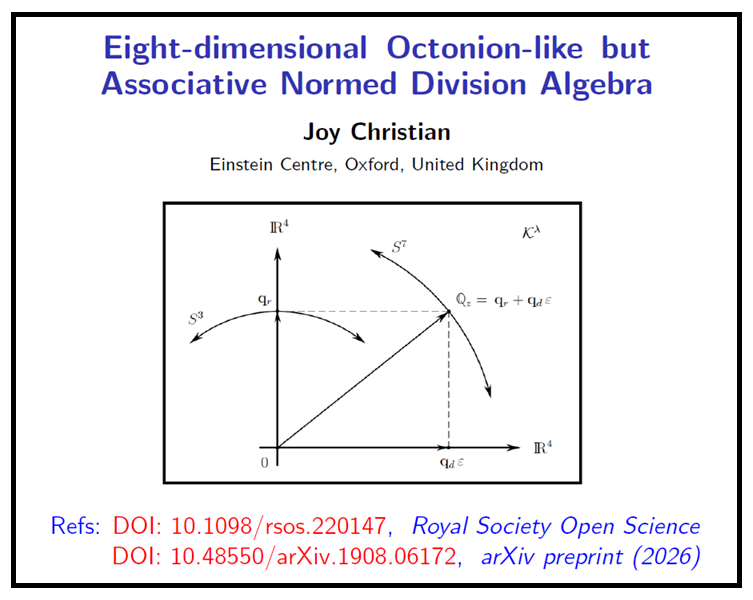
On a completely unrelated note, in your paper “Response to ‘Comment on “Quantum correlations are weaved by the spinors of the Euclidean primitives”’ you mention at the end how, following equation 2.30, that klambda is a normed division algebra with respect to the norm defined previously (the orthogonality condition). Now, I’m far from an expert in division algebras, but from what ive read a division algebra necessitates of 1) closed multiplication, 2) existence of inverses, 3) multiplicative norms and 4)closure under addition. Your specially normed klambda satisfies the first 3, but it is not closed under addition (as any sphere is not so); moreover, klambda does have zero divisors, and since the linear span of the special S7 is the full klambda, these do appear from linear combinations of those elements.
.
I understand the construction of interest is the special S7 here. But I just felt that the statement of klambda being a division algebra, in all possible interpretations, cannot be true, under what ive read. Could you explain, and point out if im in error?
120 degrees is indeed a very special angle, just as the entangled singlet state is a very special state in quantum mechanics. It is rotationally invariant and thus predicts the strongest possible correlations, maximally “violating” the bounds of +/-2 on the Bell-CHSH inequalities. All other angles characterize weaker correlations producing quantum states in the S^3 model. In other words, the values of the bounds ranging from r = 0 to r = 1 on the left-hand side of the inequalities
r ≤ ||q+p|| ≤ 2
characterize all possible entangled states, from the weakest for r = 0 to the strongest for r = 1 characterizing the singlet state.
As for the algebra K^lambda, it is a normed division algebra *with respect to my definition (2.28) of the norm*, as I have specified in the RSOS reply paper you have mentioned. You can find the proof of this in Appendix A.3 of the following paper:
Note that my definition (2.28) of the norm giving a scalar value is different from the one you will find elsewhere in the literature.
If we continue doing physics and mathematics with definitions and concepts used by “Aristotal” two millennia ago (for example), then no progress in physics or mathematics can ever be made. Progress is made by thinking differently from how others think, confined to their rigid definitions, dogmatic concepts, and lack of imagination. What I am saying is that my definition of the norm is a generalization of the definition of the norm you will find elsewhere in the literature, reproducing the usual definition as a special case.
My point is not that I disagree about the use of your special norm. The point is that, according to your own definitions, the space defined by the multivectors U and V (from that last paper you linked) is not closed under addition, which, according to the standard definition of algebra, makes the space not an algebra. For quaternions and octonions, the space spanned by the units spheres like s3 and s7 are not algebras, but the difference is that sum of their elements end up in an algebra that has no zero divisors, unlike klambda. Klambda IS an algebra, but its not a division algebra, irrespective of the definition of norm.
We can still insist on the construction being absolutely valid, the S7 could indeed be special, but that is not where my contention lies. Here, I’ll give you a clear example.
.
Let X and Y be two elements of this S7, with X= i+je and Y=j+ie, with e being your epsilon. You can check these indeed satisfy your scalar norm relation (the qr and qd are orthogonal). Now sum them, and multiply the sum by 1/2 (1-e) which is the idempotent of Klambda. You get [(i+j) + (i+j)e ]* 1/2 (1-e), which you can very easily check gives 0. The idempotent itself can also be constructed easily by summing elements of the S7, since its linear span spans the whole klambda.
.
So Klambda, even with the special norm, is not a division algebra, unless you also applied a different definition of algebra where additivity doesn’t matter.
The addition of two or more elements of the algebra K^lambda does not lead to any difficulty. In particular, the space defined by the multivectors U and V in K^lambda is closed under addition. Note that “zero” is an additive identity, and thus a part of the algebra K^lambda, just as it is in any other algebra.
The example you have constructed is essentially the same as the one I have discussed in my equations (2.7) to (2.11) of my RSOS reply paper you mentioned earlier. Let me use the following notation so you can see that. You start with X = i + je and Y = j + ie. Now, let us define W = X + Y, which gives W = (i+j) (1 + e). Next, define your idempotent as Z = 1/2 (1 – e).
You have found that WZ = 0 by applying geometric product between W and Z, which is correct, and that gives ||WZ|| = 0 on the LHS of the norm relation (2.5).
But let us now compute ||W||, which gives ||W|| = (i+j) (1 + e). This is essentially the same as my equation (2.10), apart from its scalar coefficient.
Next, compute ||Z|| = 1/2 (1 – e), which is again essentially the same as my equation (2.9). Consequently, we have ||W|| ||Z|| = [(i+j)/2] (1 + e)(1 – e) = 0.
Therefore, we have ||WZ|| = ||W|| ||Z||, even though W was obtained by adding your X = i + je and Y = j + ie. So the addition of two or more elements of K^lambda does not lead to any difficulty with the norm relation (2.5), because “zero” is an additive identity, and thus a part of the algebra K^lambda.
Thus, K^lambda is a normed division algebra with respect to the norm defined in (2.28). But of course, one has to use the definition (2.28) of norm carefully, and never make a mistake of using two different product rules on the two sides of the equation ||WZ|| = ||W|| ||Z||, as Gill and Lasenby did in their papers. What (2.28) does is projects out the pseudoscalar part of the norm so that only the scalar part remains. But this has to be done carefully, respecting the general equation (2.25). Geometrically, you can visualize this projection in two-dimensions in an x-y plane, with the y-axis representing the scalar part of the norm and the x-axis representing the pseudoscalar part. The 7-sphere S^7 is then entirely confined to the y-axis.
Sorry Joy, I don’t mean this in any conflictual sense, but your calculation here does not show that klambda is a division algebra as it is usually understood. The fact that the norm identity holds in the split-valued sense is true but irrelevant: the concrete product WZ=0 (with W and Z different from 0) is a direct algebraic counterexample to the claim that Klambda is a division algebra. If you intend a different definition for “algebra” or for “division” please state it precisely.
.
Now that I read more carefully, equation 2.60 of the RSOS paper (not the comment, the original paper) contrains further the norm of Q (the element of klambda with the orthogonality constraint) to be 1, which means |qr|^2 + |qd|^2 =1, which is one more independent real equation. Thus the dimension is not 7, but 6, so it’s not a unit 7-sphere.
The product WZ = 0 with W and Z different from 0 is not a counterexample to the claim that K^lambda is a division algebra — it is just a statement without proof. On the other hand, I have explicitly proved in Appendix A.3 of the preprint I linked above that K^lambda is a division algebra, but, of course, only *with respect to the norm defined in equation (2.28)* of the Reply paper.
As for S^7, it is a 7-dimensional sphere, not 6. This is explicit from equation (2.30) of the Reply paper. Each point of S^7 specifies a Pythagorian distance from the origin in an eight-dimensional R^8, which makes S^7 a 7-dimensional sphere, not 6. You need eight numbers to specify a point in R^8. Equation (2.30) shows exactly which eight numbers you need. You are making the same mistake that Lasenby has made in his paper.
But you don’t have to agree with me. You are entitled to your view.
Its not that i have or not to agree with you, and its not about entitlement. Please take my statements as sincere debating. I dont put a moral judgement on these ideas, like all your retractors do. If im making a mistake like you say, I really dont see where, whether in the definitions (which i checked on multiple sources) or in the calculation, but on those you agreed. Here i state my full definition of what a division algebra is:
.
“a (real) division algebra is a real vector space with bilinear multiplication and unit such that every nonzero element has a multiplicative inverse. Equivalently, there are no nonzero zero divisors.”
.
The S7 is not closed under addition, so its not a vector space. Klambda IS a vector space, but it has nonzero zero divisors. So when you say “K^lambda is a division algebra, but, of course, only *with respect to the norm defined in equation (2.28)*”, to me it means the subset of klambda with that constraint (which is the S7) is a division algebra.
.
As for the dimensionality issue, 8 coordinates minus two independent real constraints = six degrees of freedom. This is because we are fixing the radius of the sphere with that last constraint. Its a bit like saying, the set of all possible 2-spheres centered at the origin in R3 is equivalent to the set of all points in R3, but fixing the radius to a single value makes the set 2 dimensional. Equation 2.30 is exactly of the type of varying the radius of the 2-sphere in this example, since the norm is only defined up to the choice of qr^2 and qd^2.
You are right, I am only concerned with the subspace of the 8-dimensional vector space defining the algebra K^lambda that corresponds to the 7-dimensional sphere S^7. Since S^7 results from normalizing to a scalar radius, it excludes the pseudoscalar part from the outset. In other words, there are no nonzero zero divisors within S^7. The multivectors like X = 1 + e and Y = 1 – e in K^lambda play no role whatsoever in the 7-sphere framework. They are excluded by the definition (2.28) of the norm appearing in my RSOS Reply paper. So, all this talk about nonzero zero divisors is a pure distraction.
As for the dimensionality of S^7, it is clearly a 7-dimensional sphere, S^7. The mistake Lasenby first made, which you are now repeating, is to think that two constraints are required on the multivector QQ* to reduce K^lambda to S^7. That is not correct. Only one constraint, namely,
q_r q*_d + q_d q*_r = 0,
is required to reduce the multivector QQ* to the square of the scalar radius of the 7-sphere. This constraint sets the coefficient of the pseudoscalar to zero. That is all there is to it. In the notation used in my RSOS Reply paper, this constraint is equivalent to
g h + u_x v_x + u_y v_y + u_z v_z = 0,
This constraint is all that is required to reduce eight-dimensional K^lambda to the seven-dimensional surface S^7 of scalar radius embedded in K^lambda, free of nonzero zero divisors. Note that the product QQ* itself is not a constraint. It is just another multivector within K^lambda. This multivector QQ* reduces to the square of a scalar radius once the above constraint is imposed.
“all this talk about nonzero zero divisors is a pure distraction” it’s not given that you called any of these constructions (still not clear whether klambda, s7, or both) “division algebras”. As I mentioned, I was not concerned with the possible significance of the construction, but only on that claim, and it’s not even some subtle, obscure point coming out of some appendix, but rather a strong claim present directly in the title of the paper. I would not call asking for precision “distraction”.
.
I’ll have to go back to lasenby’s paper to give clearer thoughts on the matter of dimensionality. I’ll get back to you as soon as I have the time to carefully consider the proposition.
In topology and differential geometry, the normed division algebras are closely linked to parallelizable spheres S^0, S^1, S^3, and S^7, and are discussed interchangeably with them, because, clearly, only *normalized* multivectors with scalar norms can satisfy (or appear in) the scalar norm relation (2.27). So, the titles of some of my papers and statements about normed division algebras are neither unreasonable nor wrong. Moreover, it should be obvious to anyone that nonzero zero divisors play no role whatsoever in the 7-sphere framework I have proposed. They were dug up by Gill for disingenuous reasons. Therefore, all the talk about them is indeed a distraction, at least for me.
As for your continued interest in my work, I suggest that next time, if you read a critique of my work somewhere, then please first read my existing replies to it. I have published some two dozen papers and preprints, not to mention hundreds of blog posts and forum comments, over the period of two decades, where I have already provided all the answers to any conceivable questions one can have. It is not a good use of my time to keep repeating those answers for every new person who becomes interested in my work.
Dear Joy,
I’ve read lasenby’s and your reply to it again. It’s clear lasenby makes conceptual mistakes in multiple points, but i don’t see how your reply dispels the doubts i raised earlier.
You say, correctly, that the orthogonality constraint is equivalent to
.
g h + u_x v_x + u_y v_y + u_z v_z = 0
.
But note that this constraint does not constrain the norm of Q. In fact, the norm of Q is a scalar, but any scalar. This means that when we set it to 1, we further impose
.
h^2 + ux^2 + uy^2 + uz^2 + g^2 + vx^2 + vy^2 + vz^2 = r^2
.
to be
.
h^2 + ux^2 + uy^2 + uz^2 + g^2 + vx^2 + vy^2 + vz^2 = 1.
.
This is an independent constraint from the other one. Two independent constraints, 8D ambient space, 6 dimensions.
.
As for the division algebra issue, I don’t think we’ll reach an agreement there. The S7 is not a vector space, so the second part of “division – algebra” is not satisfied. Klambda has zero divisors, so the first part of “division – algebra” can’t be satisfied. Since one is a subset of the other, there’s no union or other operation on the sets that allows for both parts to be true at the same time. It’s that simple.
You are mistaken about both issues. The orthogonality constraint reduces QQ* to a scalar radius, say r. But setting r = 1 does not impose an additional constraint on the resulting space. It just shrinks the radius of the 7-sphere from r to 1. Moreover, there is no reason to set r = 1 apart from convenience. We can just leave the radius to be r without changing anything fundamental. In other words, there is only one constraint, not two, which reduces the 8 dimensions of K to the 7 dimensions of the 7-sphere.
To convince yourself, consider the set of quaternions q with radius r, which is constructed by conjugation: qq* = r^2 (try this as an exercise). This is a 3-sphere of radius r, which is a three-dimensional space embedded in R^4. Now set r = 1. Does that reduce the dimensions of the space from 3 to 2? Of course not. Setting r = 1 simply shrinks the radius of the 3-sphere to 1, making it a *unit* 3-sphere. It simply shrinks the size of the sphere from r to 1 without changing its dimensions (i.e., the number of independent variables required to uniquely specify a point in the space are still 3, not 2). Lasenby has made a silly mistake, and you are misled by it.
The second issue is largely a verbal quibble. It is true that in the un-normed algebra K, one can construct non-zero zero divisors that cannot be normalized to scalar lengths. So what? To me, that is not a very interesting observation, because it holds only for the un-normed algebra K.
What is interesting is that the algebra K, once normed, has no non-zero zero divisors. In fact, all non-zero zero divisors reduce to ordinary zero divisors once all multivectors in K are normalized to scalar lengths. Therefore, K is a *normed* division algebra.
But qq* = r^2 is valid for the whole quaternion algebra. Its solution set is 4 dimensional, not 3 dimensional. In particular, it’s a single scalar constraint on an expression with 5 variables, q0, q1,q2,q3 and r. Or in vector notation,
if q = a + v, then qq* = a^2 + |v|^2 = r^2, which is an expression with variables (a, vx, vy, vz, r).
It is you who set r=1 in the paper and called the resulting set the “unit 7-sphere.” If you do not fix r then the orthogonality locus is not a unit sphere at all but a noncompact 7 dimensional cone or an hypersurface in R8.
I think we are now repeating ourselves. From my side, the issue is straightforward: orthogonality makes QQ* a scalar, but it does not fix its numerical value. Imposing a fixed radius (whether called r or rescaled to 1) is therefore an additional scalar condition unless one proves that the radius is already determined by orthogonality. I do not see such a proof in the argument presented. At the very most, you can say that the Klambda subset is a set of infinitely many 6-spheres of all radii, like you can have infinitely many 3-spheres inside the quaternions.
On the algebraic side, normalization does not remove zero divisors. So from my perspective the structural questions remain.
In any case, I don’t think we’re going to reach agreement here, so I’ll leave it at that. I appreciate the exchange very much as usual Joy, and I hope that if I have more questions on other parts of your work I can still post them here.
I am not concerned about either of the two issues you have raised because both are non-issues in my view. But I understand that sometimes issues like these are not easy to follow from my writings. If an expert on GA like Lasenby can stumble on some of them, then others may also have difficulty understanding them. Therefore, I plan to add a new appendix to one of my existing papers, where I will make my point of view clearer and also address the two issues you have raised.
They address the misinterpretations of its main results by Lasenby and others. In Appendix D, I prove once again that the algebra K^lambda is a normed division algebra, and the sphere it embeds is a 7-sphere. In particular, I demonstrate that the embedded surface cannot be interpreted as anything but a seven-dimensional sphere. Moreover, the so-called “nonzero zero divisors” in K^lambda cannot be normalized to give scalar lengths, and therefore they are not part of the *normed* algebra. They are excluded by the criterion of scalar-valued normalization explained in the paper.
Then, in Appendix E, I explicitly construct a linearly independent basis for its tangent space, demonstrating that this 7-sphere is parallelizable, which further consolidates that the surface embedded by the algebra is a genuine 7-sphere.
Finally, in Appendix F, I prove that there are no non-zero zero divisors in the *normed* algebra K^lambda.


^2 = 2^2\times 4^2 = 64}}")
\,(y_1^2 + y_2^2) \,=\, (x_1^{}y^{}_1 - x^{}_2y^{}_2)^2 + (x^{}_1y^{}_2 + x^{}_2y^{}_1)^2\,=\,z_1^2 + z_2^2. \ \ \ \ \ \ \ (1)")

\,(y_1^2 + y_2^2 + \dots + y_n^2) \,=\, z_1^2 + z_2^2 + \dots + z_n^2. \ \ \ \ \ \ \ (2)")
}}")
}}")

")
")


I recently became interested in Garret Lisi’s E8 theory. There are a lot of commonalities between that and your octonion sphere model. What caught my attention is his description of spin as “gravitational charge” (referring to cartan theory), and the higgs field basically being the torsion of spacetime. Ever looked into it? I admit I have like 10% of the required math knowledge to look at it beyond his descriptions in a ted talk, so perhaps before diving into it more and start researching the stuff i need to know i was wondering if you have any thoughts on that, if at all.
Thank you for all your answers Joy.
I have met Gerret Lisi. I was at the 2011 FQXi conference where he gave a talk on his E8 theory. His work is interesting, but I haven’t spent time on it beyond listening to his talk at that conference because my focus is elsewhere. I don’t know how much Geometric Algebra Lisi uses, but David Hestenes was also present in his FQXi talk, and Lisi gave credit to Hestenes for inspiration. Sabine Hossenfelder was also at that FQXi conference and, if I recall correctly, she has made a video about Lisi’s theory, which may help you.
Dear Joy,
quick question. In the paper “Bell’s Theorem Versus Local Realism in a Quaternionic Model of Physical Space” I don’t understand how you derived eq. 25. In particular I don’t understand how exactly the angles ne and zs are assigned or what their relationship is, as if we set such angles both to pi/2 (with k=+1), or some interval around pi/2 (like 80-100°) the norm of |P+Q| becomes larger than 2, which is not allowed since on S3 this norm is bounded by 2.
Hi Sandra,
Eq. 25 is not derived. It is postulated. It is an ansatz. I have made it up, because it works.
The angles ne and zs are constrained by the inequality 28, which follows from the triangle inequality 23. Thus, ne and zs can take any angular values subject to the constraint 28. As long as the inequality 28 is satisfied, the norm will not exceed the value of 2.
I see. Is there an intuitive geometric idea behind ne and zs? In your paper you mention n can be thought of as a measurement direction, z as a “reference” vector at another point of S3 (which i personally think of as either i,j or k), and e and s are related to the spin system. In particular you mention that s can be thought of as the vector dual to the bivector Is representing the spin of the combined pair, but isn’t that bivector by definition 0 since angular momentum is conserved (e1=e2)? Also I’m struggling to geometrically relate all of this to the fact that certain angles are essentially forbidden.
You are struggling because it is not an elegant approach like that based on the even subalgebra of the Geometric Algebra Cl(3, 0) or a quaternionic 3-sphere. I used that “ugly” approach in that paper to make contact with Pearle’s non-Clifford-algebraic approach [ see Ref. 34, where I cite his famous paper ], which allows numerical simulations of the singlet correlations.
No angles are forbidden by the constraint 28. What is forbidden are certain *relations* between the angles ne and zs. If these relations are admitted, then they would throw us outside the geometry of the 3-sphere, because including them would violate the triangle inequality 23, which must be respected to respect the geometry of the 3-sphere.
By “composite pair” in the paragraph above Eq. 23, I mean just “spin-1 and spin-2” regardless of the net values of their spins, not their singlet state defined in Eq. 9. The net angular momentum of the two spins in the singlet state would indeed be zero.
Dear Joy,
i studied more carefully your “Symmetric” paper. In it, you show the example that on a moebius strip, the intrinsic angle Nas is related to the extrinsic angle (Bas) by B=pi(1-cosNas). You also derived the linear correlation using B as E(a,b) = -1 + B/pi.
.
Then, I noticed that the linear correlations derived by Bell in his Toy model has the form
E(a,b) = -1 + 2Alpha/pi. Obviously there’s a very clear similarity here between the two correlations, with B = 2Alpha. Tell me if this is the correct way to think about it:
.
If we assume R3, there’s no twist, and the correlation is the linear one of Bell. If we assume S3, there’s a twist, then we need to relate Theta to the intrinsic twist angle Nas. The factor of 2 comes from the double covering of SO(3). So doing the substitution Alpha = pi/2 (1-cosNas) we obviously end with E(a,b) = -cos(Nas).
.
There’s more. The relation psi=pi(1-cos(theta)) derives from the holonomy on the Hopf Projection on S2, with psi is the phase on the S1 fibers after a full loop and theta is the polar angle on S2 where the loop is constructed. So if we make theta=pi/2, we’re at the equator, where the twist becomes a full pi angle, exactly like in the moebius strip. This justifies making the substitution psi = Nas as an intrinsic angle. Then from the relation alpha = pi/2(1-cosNas) it becomes clear that Nas is equal to alpha, that is, we can relate the angle between detectors with the angle in the twist of S1! Hence,the non-linear correlations!
.
I think this makes a lot of sense, but I wanted to ask you if my understanding is indeed correct.Months thinking about S3 left me in the clouds a bit too much.
I think you are talking about “Dr. Bertlmann’s Socks” paper, not the “Symmetric” paper.
Your understanding above is essentially correct, as long as you keep in mind that the toy example is not the real thing. The Mobius strip is not a 3-sphere. At best, it is just one of the S^2 worth of circles that make up the 3-sphere. What is more, the Mobius strip is not *orientable*. A consistent sense of handedness cannot be specified on a Mobius strip because there is a twist in it. By contrast, a 3-sphere is orientable and can be parallelized to specify a consistent sense of handedness over the entire sphere, without ever having to change the “hand.” As long as you keep in mind that the Mobius toy example only provides an analogy to help our intuition, you will be fine.
Happy Easter Joy!
Why exactly is the orientability important here? A cosine correlation can be derived regardless. I know orientation is your hidden variable Lambda, but even that drops when the two measurement functions are multiplied.
Happy Easter! We do not live in a 2-dimensional, one-sided world of a Mobius strip. As I have argued, we live in a 3-dimensional world of a 3-sphere, which differs from a flat Euclidean space R^3 only by a single mathematical point at infinity. Moreover, an ordinary unit 3-sphere defined by the equation w^2 + x^2 + y^2 + z^2 = 1 and embedded in R^4 cannot be charted by a single coordinate system without encountering a singularity somewhere, usually chosen to be at the north pole. However, a 3-sphere is parallelizable with quaternions, which renders it a flat, orientable set of unit quaternions. Meaning, unlike the ordinary 3-sphere, a quaternionic 3-sphere can be charted by a single coordinate system with a fixed handedness without any discontinuities, singularities, or fixed points. This is important because excluding a single point (say, at the north pole) would render it topologically equivalent to a flat Euclidean space R^3 — S^3 minus a point is equal to R^3. And we know that measurements within R^3 cannot reproduce strong quantum correlations, as proved by Bell’s theorem. Thus, orientability is a necessary and sufficient criterion for a 3-sphere to be able to reproduce strong quantum correlations.
Joy,
Reading through the pages of your blog I’ve seen you also used a different derivation for the triangle inequality, where you derive |cos(ae)| >= 1/2 sin^2(theta). Now this to me is a more rigorous result, as this function itself does constraint the sum of two quaternions to 2 for all angles.
.
So I’ve tried simulating it in excel, and indeed the result is the correct correlation. But I was wondering how I should interpret geometrically this constraint. I realize it essentially relates “projected” quantities (vectors instead of bivectors) to the geometry of a 3-sphere. But is there a direct correspondence to, for example, the Hopf projection? Could theta be a polar angle on the base space S2, and ae0 the angle on the fiber? Or perhaps some other interpretation?
.
Another question as well. The initial state (e0, theta) gives the final measurement result as sign(cos(ae0)). But for some angles theta this “metric” returns zero, so you say the state for which the metric is zero does not exist on S3. But of course for a given (e0, theta) whether the metric is zero or not depends on the measurement direction a, and as this varies different states are said to “not exist”. How should I interpret this geometrically, perhaps related to the projection picture? For a given theta, why are some angle relationships between e0 and a constrained? For example, you mention that at theta=pi/2 most of e0 and a are orthogonal to each other, but if we sub in the constraint this value we get |cos(ae)| = 0.5, which means ae=60°.
Hi Sandra,
The approach with the constraint |cos(ae)| >= 1/2 sin^2(theta) was phenomenologically motivated. Its purpose was to produce numerical agreement with the observed correlations. It is pointless to force a geometrical interpretation on such a crude approach, or compare it with the elegant approach using a Hopf fibration of the 3-sphere.
Joy,
I don’t think it is pointless. Without such a geometrical interpretation people won’t stop accusing it to be simply a detection loophole model. It’s not enough to just say “it follows the topology and geometry of the 3 sphere” without directly creating a correspondence between them. At least, that is what I’m concerned with since I want to make it into a video, but I’ve been stuck on these details for months.
In Section III G of the following paper (open access), I discuss what is wrong with Pearle’s detection loophole model, and then make a detailed comparison with the quaternionic S^3 model:
https://ieeexplore.ieee.org/document/9693502
In that section, you will see that the geometrical relation between the two models is quite involved and requires considerable effort to identify the flaw in the detection loophole argument. Most people like Gill are mathematically too incompetent to see the flaw in Pearle’s model. You, on the other hand, are one of the very few people who are making an effort to understand the S^3 model. I appreciate that because it is hard work. But, unfortunately, the geometrical and topological subtleties of the S^3 model are too difficult to explain in online discussions, such as in your effort to make a YouTube video about them.
Note also that the comparison of the two models requires a different constraint derived from the triangle inequality within S^3, not the one with the phenomenologically motivated sine function you have noted above.
Dear Joy,
one more question about the “Bertlmann” paper, which came to me after more scrutiny. In the toy model you state that the relation between the extrinsic, “cylindrical” angle on the strip and the intrinsic twist angle, seen from a cross-sectional view, is beta(ab) = pi(1-cos(nab)). But since the twist is uniformly distributed along the entire length of the strip, the actual relationship is linear, more specifically beta(ab) = 2n(ab).
.
The relation you write is an holonomy relation, but I’m not sure how you square the two together.
Angle is always defined in terms of the arc length of a circle, not a straight line. So, the relation beta(ab) = 2n(ab) you wrote down is incorrect. The correct relation between the two angles is beta(ab) = pi(1- cos(nab)).
Ooh, so it’s due to the fact that the strip is not straight but curved! Obvious in hindsight. Thank you Joy.
Dear Joy,
sorry to bother you on the same issue again. I’ve been trying to find a derivation of the relation beta(ab) = pi(1- cos(nab)) for a moebius strip for months now, but i could not understand how it is done (despite your previous answer on the matter). Since this kind of formula is found when dealing with areas and curvatures, i tried looking up integrals for the same relation but for flat surfaces with torsion like the moebius strip, but they all give a linear result. Could you provide a resource to understand how to derive this relation, on the strip specifically? In your paper you simply state “for the well known properties of the moebius strip” which unfortunately wasn’t much of help for me.
Hi Sandra,
I am not sure why you are wasting so much time on that toy example. It is not a model for the singlet correlations observed in the real world. The purpose of the toy example is to give us an intuitive understanding of a characteristic feature of the geometry of the quaternionic 3-sphere in the real world. I have warned in my papers not to take the toy model too seriously. In particular, the relation beta(ab) = pi(1- cos(nab)) cannot be derived for a Möbius strip. It postulates a physical characteristic of the toy world that a two-dimensional Alice and Bob are assumed to inhabit. That is why I have stressed that the relation beta(ab) = pi(1- cos(nab)) is the defining relation of the Möbius world of Alice and Bob. It has to be accepted, not derived, for the illustration to work.
Dear Joy,
the reason being that I want to understand the reasoning in your papers. A toy model is supposed to present a simplified, yet not necessarily comprehensive or even widely applicable, version of a model. If I understood the toy model completely, then I would feel more confident trying to understand the whole model, wary of the limitations of the toy model itself. The problem with just giving out mathematical relationships ad hoc without fully justifying them, even on a matter of principle, leaves more questions than answers, which defeats the point of creating a toy model. I’m not sure why you question me questioning the derivation, I just didn’t understand it. Should I be held at fault for not understanding “defining relation” as “we are just assuming this holds”?
Given that I’m much more of a visual person rather than a math one, I can now understand the relation pi(1- cos(nab)) as a torsion not uniformly distributed on the strip, centered on the midpoint between a and b. But that seems to mean the choice of a influences the possible choice of b, so by accepting that relation we are introducing non-locality in the strip (there’s no global distribution of torsion that works for all a and b). Perhaps you have objections here, but please don’t just say “ignore the toy model”. I’ve been passionately reading tons of posts on your work, by many people, and I understand most of your critics to be wrong on many points they make. Just to make an example, I immediately recognized that the “sign error” many of them talked about is in fact their misunderstanding of the idea behind the change in orientation. One thing they are not wrong about though, is that sometimes your writing style can be a bit cryptic, especially to those without years of experience on GA, topology and GR.
Hi Sandra,
There is no deep issue to resolve here. By hypothesis, the relation beta(ab) = pi(1- cos(nab)) *defines* the toy geometry of the two-dimensional world Alice and Bob live in; just as, by hypothesis, we live in a three-dimensional geometry isomorphic to a quaternionic 3-sphere. The relation beta(ab) = pi(1- cos(nab)) is not a standard property of a Möbius strip. So, it cannot be derived. But there is no need for its derivation, since we are working within a hypothesised toy model. I think what you are missing here is not mathematics, but the logic behind the toy model.
Hello Joy,
I’ve come to terms with your toy model. Unfortunately, I don’t think it helps at all with anything, but that’s just my very humble opinion. After reading and reading, ive come to the conclusion that the most fundamental thing in all of this matter about Bell’s theorem, QM correlations and so is a single property of S3, that it is a non trivial bundle. The central argument for which Bell’s inequalities are considered inapplicable, here and on many posts on sciphysicsforum, is the impossibility of measuring different settings on the same particle pair. This in turn means the outcomes corresponding to the same setting cannot be factorized through different integrals, thus making deriving the classical bound impossible. Another way that this argument was put in was that the additivity of expectation values is not respected across different settings.
To me, all these arguments are really just one argument, that the distribution p(lambda) is different for different setting pairs, preventing the existence of a global joint distribution valid for all settings. This is exactly in line with some critiques by Karl Hess, and Fine’s result (whereby the existence of such a distribution = validity of the CHSH inequality).
I’ve also learned that, through yours and tsirelson’s equivalent derivation, that non commuting observables are what cause an obstruction in QM to the existence of a global joint. In particular, when viewed as a topological obstruction, no global joint = no global section on the outcome space. I’ve also learned that a non trivial bundle provides exactly such a lack of global section. This mirrors the simple fact that the same path in SO(3) can lift to two different paths on SU(2). From the point of view of R3 outcomes really do seem to depend on the distant setting (they look context dependent), but that is simply because we ignore the full specification of the state, which must include the relative points on the fibers for the same bloch vector. Likewise, we can’t know which SU(2) path was taken from a single rotation; but we can infer it through comparison of two different rotations of the same state. The response functions depend on the lift. Thus, a joint probability on the base implicitly pretends that all outcome-determining variables are functions of basepoints only; if the true ontic dependency lives in the fiber (lift) and there is no global, consistent way to choose a lift over the whole base (no global section, which is guaranteed for a jon trivial bundle), then we cannot compress the model to a single, context-independent probability on the base that reproduces all lift-dependent statistics.
I’m not sure you’ll agree with my conclusion here; but this has been the clearest way for me to make sense of all I’ve read. I also believe that this helps with the conceptual issues I’ve had with your simulations. The “detector loophole” can likewise be framed in terms of differing joints for different settings; when elements of one distribution are used for a pair of settings which uses a different distribution, some of such elements may not be present in that distribution. Thus the need to specify a full list of “initial states” for setting pairs like in your simulation.
Overall, I think I will take a break from studying these matters. On one hand, im tired of the vitriol directed at both parties in the matter, which also has made it very hard to follow through with your proposed experiment (which would settle the matter once and for all), even thogh initially i did find interested individuals; on the other hand, I feel like I don’t really have the cognitive energies to change once again the way I think about all of this, which i hope i made with sufficient precision above.
Joy, with my previous post I didn’t mean that I dont value your input in the matter. I want to make that clear since I realized it could have been interpreted that way.
Hi Sandra,
Understood.
I am happy to answer any genuine technical questions about my work. But only about my own work. I have wasted enough time addressing bogus claims about my model by incompetent non-physicists such as Gill and Aaronson, so I am no longer inclined to answer any issues that arise from their online, non-peer-reviewed comments. As you may know, the Royal Society has now published my detailed rebuttal to Gill’s bogus claims about my work:
https://royalsocietypublishing.org/doi/10.1098/rsos.220147
This has allowed me to expose just how incorrect and incompetent all of the critics of my work have been. Consequently, I am no longer inclined to fight a proxy war with them, via you or anyone else. I have more serious work to do, and such proxy wars (however well-intended) are a huge distraction from my ongoing research.
My post above did not stem from either Gill, Aaronson or any other of your critics. It is my observations only on what your work implies; the main point i was trying to make is that mathematically, those expectation values are different integrals over different setting choices (hope we agree here). If we assume the global joint p(lambda) over outcomes exists and is the same for all settings, then mathematically for the large N limit the sum of those integrals is the same as the integral of the sum. Many posts of Michel Fodje, which you endorsed, point out that Bell’s inequalities involve dependent terms like A1B1 + A1B’1 + A’1B1 – A’1B’1, which can indeed be factorized. For independent terms, which would be the case for experiments since we can only measure two settings at a time, the correct expression is A1B1 + A2B’2 + A’3B3 – A’4B’4. But in the large N limit, if we assume those As and Bs are drawn from the same fair sample, the two expressions are indeed equivalent. Thus, my observation that since QM violates the inequality, then it means, in view of the above, that the As and Bs are NOT drawn from the same sample for the different integrals. Which means either 1) outcome dependence (A depends on B and viceversa, i.e. non locality) or 2) p(lambda) being a “function” of settings. What I’m proposing, in view of your own results, is that condition 2) does not necessarily mean superdeterminism; that is only the case if we insist on making A,B functions of the base only. But on S3, what looks like superdeterminism in S2 simply stems from the topological properties of S3, namely the lack of a global section. Functions on the whole space (like your own As and Bs) are not limited in this way. That is what I tried to get across, and what I hoped to get your feedback on. I simply tried to find a way to restate your work in a different manner.
Hi Sandra,
Ok, you have now expressed your point more clearly, and it is worth thinking about.
To begin with, you are quite right to point to the lack of a global section in the fibration of S^3 as the root cause of the differences that arise in the strength of the correlations when measurement results are charted on S^2 versus S^3.
However, your suggestion that this lack of a global section should be interpreted as making the probability density p(lambda) depend on settings is problematic, because a setting-dependent function p(lambda | a, b), in fact, implies a more subtle form of non-locality. Clauser and Horne have explained this nicely in footnote 13 of their paper “Experimental consequences of objective local theories,” Phys. Rev. D., vol. 10, pp 526 – 535 (1974). So, your observation concerning the lack of a global section on S^3 does not let you escape a form of non-locality, if you want to think of strong correlations in terms of Bell inequalities.
But independently of S^3, the real reason why strong correlations violate Bell inequalities has to do with the assumption of linear additivity of expectation values, regardless of the setting-dependent or setting-independent probability density p(lambda). As is well known, linear additivity holds in quantum mechanics, making it a non-local theory. On the other hand, while we must assume setting-independent probability density p(lambda) to preserve strict locality, there is no reason to assume linear additivity of expectation values in hidden variable theories. I have explained this in considerable detail in my latest analysis of Bell’s argument: https://arxiv.org/abs/2302.09519
Dear Joy,
hope you had a wonderful holiday. To start the new year, i made this small simulation:
https://output.jsbin.com/zefayihecu
It helped me understand a little better your work. It uses the |cos(alpha)|>1/2 sin(theta) function to discard non existent states. There’s a little ? box you can click to show my understanding of this function.
The angle slider also slides along the fiber of the hopf fibration, which i understand is equivalent to fixing S for a spin vector with coordinates (x,y,z,S) and show how that vector “sees” the orientation with respect to the measurement vector (which is why the spheres behave like they do). Then the simulation runs by picking a uniform sample of points over all directions, and also picks over a uniform choice of theta. The whole thing is basically a tomography of the 3-sphere projected down onto a 2-sphere.
Hope you’ll find this interesting, it took a while to get going. You can also change the colors.
I might have messed up the link (i created it not logged in). It’s still viewable, but to get it to full screen you’d have to click on the little arrow with “live preview”. Otherwise try this link https://jsbin.com/luwadov which should stay working.
Thanks, Sandra, for the simulation.
I was able to run it for a while, then it was not visible.
I can view it again at a new link. I will play around. It is interesting.
Sorry again, whish i could just edit my previous answers. The site i’ve used is convenient for running the code immediately at the link, but it seems it has often issues.
This is my GitHub page
.
https://github.com/Sandra-Lu-Lang/Simulation/blob/main/simulation%20FINAL.html
.
you can either copy-paste the file to a text file and save it as html, or you can directly download the file from the page. As html code, it works on any browser.
That is better. I now have the simulation working in my browser.
I’ve added support for changing the threshold function, you can check it by downloading the new version at the same link. One interesting thing i’ve noted is that we would expect the PRBOX type correlations to arise for setting theta to 90° and the metric l0 to 1 (since g(u,v,s)>l0 * sin^2(theta)). But, in the simulation, the colored bands become always antipodal earlier than that, meaning the grey exclusion area becomes big enough so that the bands can never overlap with the same color and the opposite color at the same time (forcing always correlated/anticorrelated outcomes). I’m not sure what feature of this particular simulation causes this, and how to interpret it. The way the shader currently works is essentially a flat texture 2PI long, which is wrapped around the sphere and made to flow up and down changing angles. I wonder if I could fix this particular issue by allowing the band length to change with the metric prefactor, so at 1 it would be twice as big stretching with it the colors, but then I would not recover Bell’s models at metric set to 0, as that would mean the texture would have 0 size…
Thanks for the update, Sandra.
I think you probably mean Pearle, not Fine. The theta function was Michel Fodje’s invention, whereas the other threshold function was extracted from Pearle’s paper.
Unless you have some other function in mind when you say Fine, which I’m not aware of.
Yes, obviously I meant Pearle. I have no idea why I mixed him with Arthur Fine. Thanks
Sandra, I noticed that the simulated correlations always turn out to be a little weaker than those predicted by quantum mechanics. This suggests to me that there is a systematic bias in the simulation (or a small bug in the code). Not a big problem, because the simulation does demonstrate what you intended it to, but there is room in it for fine-tuning.
Yes I’m aware. The bias comes from the fact that the mask is only applied in intervals of 1°, as the slider can only change in those steps, which doesn’t allow for a perfectly uniform average over all angles. To make it more accurate I would have to increase the steps and allow for more decimal places, but that comes at severe computational cost especially for an html file. I’m happy though that you played around with it a bit.
.
What do you say about my reading of theta as a tomography? It came from noticing that interpreting |cos(alpha)| as a state density would mean it comes from the jacobian, as the uniform measure on S3 is pushed forward on S2. The analogy i thought of is that of mercator projections of the globe, which brings with it distortions… so if we were to use simply a flat coordinate chart to measure areas, we would conclude greenland is much bigger than it actually is. Instead, sliding theta, in this analogy, would allow us to rotate the globe on this projection an put greenland “on the equator” to judge its true size.
I’m aware that in your paper you mention that theta links two “disconnected” S2s on S3 made by the bivectors Ia and Ib, but I couldn’t quite understand that geometrical reading, as both Ia and Ib are pure quaternions and lie on the equator of S3, meaning they form a single S2 together.
I like the idea of reading theta as a tomography. That gives a new, perhaps more useful perspective in practice. It would be a challenging task to match your tomographic perspective with the actual mathematics of the Hopf fibration, which also maps the points of S^3 to the points of S^2, by a many-to-one function. That is the map Hopf discovered in 1931. At the moment, it seems to me that these are two distinct ways of looking at the same physics, but not necessarily at the same mathematics.
Joy, the simulation helped me get more in-depth insights into its method. What I’ve noticed is that the correlation works out whatever threshold function clamped between 0 and 1 you provide it. For example, setting the exclusion function to be |cos(alpha)|>= (1+cos(theta))/2 still reproduces the correlations of QM. This is a result of the fact that ||q+p|| f(sz). Now, the question is, why set that norm to that expression, since in theory 0<||q+p||<2, but that expression is bounded like 1<1+sin^2(ne) + f^2(zs)<2, unless f(zs) is imaginary. We are restricting the chord length between q and p to be less than 120°, although q and p seem like independent unit quaternions. We are not taking a uniform distribution of unit quaternions on S3. You do say that e0 is the vector of one of the two spins, while s0 represents the pair, so maybe they are related in a non-trivial way, but I'm not sure i follow.
Hi Sandra,
Pearle’s distribution (or threshold) function is not unique, and Michel Fodje’s sin(alpha) choice is just as good, if not better, as your simulation confirms. In fact, there are many solutions to how Pearle set things up in his paper. Moreover, sin(alpha) and cos(alpha) are essentially the same function, apart from a 90-degree phase difference, which does not play any significant role in any simulation. So, it is not surprising that you found several other possibilities for a threshold function. These possibilities will be narrowed somewhat if you can fine-tune your simulation, but still, many options will remain. Note that your simulation, or any simulation for that matter, is not a local hidden variable theory by itself. For that, a deeper theoretical understanding is required, and that is what is provided by the geometry and topology of the 3-sphere — at least in my view.
Yes and that’s what im interested in understanding. Could you clarify better what is the intuition behind your choice for ||q+p|| to be bounded by 1 from below? I’m referring to your derivation of the threshold through the triangle inequality on the 3-sphere. You mention vectors e0, s0, and a reference vector z, and how one can be thought of as a single spin vector, while s0 refers to the pair… I just could not understand this.
The quaternions q and p with ||q+p|| < 1 will not be in S^3, which is the set of all *unit* quaternions. So we require the quaternion q+p to be a unit quaternion as well, belonging to S^3. Consequently, the bounds on the sum of q and p are
1 < ||q+p|| < 2,
even though the triangle inequality allows the lower bound on the sum to be < 1.
The quaternions i and -i are in S3, yet their sum is 0. For q+p to be a unit quaternion we would require its norm to always be 1, which means taking q and p to be exactly at 120° from each other. This does not allow values greater than 1 though, since as soon as |q+p| is more than 1 then its not a unit quaternion anymore. But if we dont allow those values, then for the expression with f^2(zs) it would mean setting both angles to 0, including theta in the simulation, and we would only have |costheta| more than 0 always, which is bell’s model. I also dont see a clear reason why q+p ought to be a unit quaternion, but that’s perhaps because i havent understood what zs0 represents here with respect to ne0.
You have misunderstood my comment. I did not mean that q+p must always have a unit norm. Rather, the norm ||q+p|| of the sum q+p must be at least 1 and never less than 1. But it can be greater than 1, and up to twice as much. The precise relation is:
1 ≤ ||q+p|| ≤ 2,
where the upper bound of 2 is set by the triangle inequality. This relation, with the lower bound of 1 instead of 0, is a 3-sphere counterpart of the quantum mechanical entangled singlet state, with several options for the threshold function.
Ok, but why? This is essentially stating p,q belong to S3 and Re(qp*)>0.5. As I said earlier, its a restriction on the state space. Again, this might be hard on me because i dont have a clear understanding of what sz0 represents.
Do you mean it in the sense of the exact counterpart of 1/sqrt2 (|10> – |01>)?
In that case, the normalized state would be q + p / |q+ p|, but even here i dont see ang reason why |q+p| cant be less than 1.
I think what you are missing is that there are two things at play in the model: (1) the geometry of the quaternionic 3-sphere, and (2) the correlations prediction of which quantum state we are trying to reproduce within the model. So, it is not just a matter of the geometry of the 3-sphere.
Now, in the relation
1 ≤ ||q+p|| ≤ 2,
the upper bound of 2 is fixed for all quantum states by the triangle inequality and the fact that both q and p are of unit norm. That leaves the value of the lower bound open, and it depends on the correlations prediction of the quantum state we are trying to reproduce. Recall that the quantum mechanics of the entangled singlet state predicts the strongest possible correlations. So, for the singlet state, which is of primary concern in my paper you are referring to, the lower bound on the above relation would have to be of the most restrictive value, which is 1, in order to reproduce the strongest possible correlations.
For any other quantum states, which are not considered in that paper, the lower bound on the above relation can be less than 1, and consequently, weaker correlations will be produced in the simulation for those states. In other words, the lower bounds in the range of 0 to 1 can be viewed as representing the correlations predictions of different quantum states.
You can test what I am saying in your simulation. For example, set the lower bound to 0.3 or 0.5 instead of 1. You will find that the correlations are then weaker than those produced by the singlet state. They will not be as strong as -cos(a, b).
I see. That’s an interesting way to put it. So you are saying there is something about the geometry of the singlet state that forces the lower bound to be 1. But what would that be?
The singlet state is rotationally invariant in three dimensions — i.e., in R^3. We are not discovering this. This is quite well known. It is this geometrical property of rotational invariance of the singlet state that is responsible for the strongest possible correlations predicted by this state.
What is new (discovered by us) is that in four dimensions of R^4 in which the quaternions 3-sphere is embedded, this property is reflected in the simple angular relationship between the quaternions q and p whose norms are bounded as
0 ≤ ||q+p|| ≤ 2.
Think of the quaternions q and p as two four-dimensional vectors in R^4. As the angle between q and p varies from 180 to 120 degrees, the correlations change from the weakest to the strongest, with the strongest correlations produced for the angular difference of 120 degrees, which is equivalent to the lower bound of 1 instead of 0 in the above inequalities.
Dear Joy,
I’ve thought a little bit about your last reply, but have not reached a conclusion yet. Truth be told, 120° is a special angle on all spheres, as it represents the maximum angle for the sum of any two unit vectors to lie outside or on the surface of a unit sphere… but I haven’t connected all the dots.
.
On a completely unrelated note, in your paper “Response to ‘Comment on “Quantum correlations are weaved by the spinors of the Euclidean primitives”’ you mention at the end how, following equation 2.30, that klambda is a normed division algebra with respect to the norm defined previously (the orthogonality condition). Now, I’m far from an expert in division algebras, but from what ive read a division algebra necessitates of 1) closed multiplication, 2) existence of inverses, 3) multiplicative norms and 4)closure under addition. Your specially normed klambda satisfies the first 3, but it is not closed under addition (as any sphere is not so); moreover, klambda does have zero divisors, and since the linear span of the special S7 is the full klambda, these do appear from linear combinations of those elements.
.
I understand the construction of interest is the special S7 here. But I just felt that the statement of klambda being a division algebra, in all possible interpretations, cannot be true, under what ive read. Could you explain, and point out if im in error?
120 degrees is indeed a very special angle, just as the entangled singlet state is a very special state in quantum mechanics. It is rotationally invariant and thus predicts the strongest possible correlations, maximally “violating” the bounds of +/-2 on the Bell-CHSH inequalities. All other angles characterize weaker correlations producing quantum states in the S^3 model. In other words, the values of the bounds ranging from r = 0 to r = 1 on the left-hand side of the inequalities
r ≤ ||q+p|| ≤ 2
characterize all possible entangled states, from the weakest for r = 0 to the strongest for r = 1 characterizing the singlet state.
As for the algebra K^lambda, it is a normed division algebra *with respect to my definition (2.28) of the norm*, as I have specified in the RSOS reply paper you have mentioned. You can find the proof of this in Appendix A.3 of the following paper:
https://arxiv.org/abs/2205.11372
Note that my definition (2.28) of the norm giving a scalar value is different from the one you will find elsewhere in the literature.
If we continue doing physics and mathematics with definitions and concepts used by “Aristotal” two millennia ago (for example), then no progress in physics or mathematics can ever be made. Progress is made by thinking differently from how others think, confined to their rigid definitions, dogmatic concepts, and lack of imagination. What I am saying is that my definition of the norm is a generalization of the definition of the norm you will find elsewhere in the literature, reproducing the usual definition as a special case.
My point is not that I disagree about the use of your special norm. The point is that, according to your own definitions, the space defined by the multivectors U and V (from that last paper you linked) is not closed under addition, which, according to the standard definition of algebra, makes the space not an algebra. For quaternions and octonions, the space spanned by the units spheres like s3 and s7 are not algebras, but the difference is that sum of their elements end up in an algebra that has no zero divisors, unlike klambda. Klambda IS an algebra, but its not a division algebra, irrespective of the definition of norm.
We can still insist on the construction being absolutely valid, the S7 could indeed be special, but that is not where my contention lies. Here, I’ll give you a clear example.
.
Let X and Y be two elements of this S7, with X= i+je and Y=j+ie, with e being your epsilon. You can check these indeed satisfy your scalar norm relation (the qr and qd are orthogonal). Now sum them, and multiply the sum by 1/2 (1-e) which is the idempotent of Klambda. You get [(i+j) + (i+j)e ]* 1/2 (1-e), which you can very easily check gives 0. The idempotent itself can also be constructed easily by summing elements of the S7, since its linear span spans the whole klambda.
.
So Klambda, even with the special norm, is not a division algebra, unless you also applied a different definition of algebra where additivity doesn’t matter.
The addition of two or more elements of the algebra K^lambda does not lead to any difficulty. In particular, the space defined by the multivectors U and V in K^lambda is closed under addition. Note that “zero” is an additive identity, and thus a part of the algebra K^lambda, just as it is in any other algebra.
The example you have constructed is essentially the same as the one I have discussed in my equations (2.7) to (2.11) of my RSOS reply paper you mentioned earlier. Let me use the following notation so you can see that. You start with X = i + je and Y = j + ie. Now, let us define W = X + Y, which gives W = (i+j) (1 + e). Next, define your idempotent as Z = 1/2 (1 – e).
You have found that WZ = 0 by applying geometric product between W and Z, which is correct, and that gives ||WZ|| = 0 on the LHS of the norm relation (2.5).
But let us now compute ||W||, which gives ||W|| = (i+j) (1 + e). This is essentially the same as my equation (2.10), apart from its scalar coefficient.
Next, compute ||Z|| = 1/2 (1 – e), which is again essentially the same as my equation (2.9). Consequently, we have ||W|| ||Z|| = [(i+j)/2] (1 + e)(1 – e) = 0.
Therefore, we have ||WZ|| = ||W|| ||Z||, even though W was obtained by adding your X = i + je and Y = j + ie. So the addition of two or more elements of K^lambda does not lead to any difficulty with the norm relation (2.5), because “zero” is an additive identity, and thus a part of the algebra K^lambda.
Thus, K^lambda is a normed division algebra with respect to the norm defined in (2.28). But of course, one has to use the definition (2.28) of norm carefully, and never make a mistake of using two different product rules on the two sides of the equation ||WZ|| = ||W|| ||Z||, as Gill and Lasenby did in their papers. What (2.28) does is projects out the pseudoscalar part of the norm so that only the scalar part remains. But this has to be done carefully, respecting the general equation (2.25). Geometrically, you can visualize this projection in two-dimensions in an x-y plane, with the y-axis representing the scalar part of the norm and the x-axis representing the pseudoscalar part. The 7-sphere S^7 is then entirely confined to the y-axis.
Sorry Joy, I don’t mean this in any conflictual sense, but your calculation here does not show that klambda is a division algebra as it is usually understood. The fact that the norm identity holds in the split-valued sense is true but irrelevant: the concrete product WZ=0 (with W and Z different from 0) is a direct algebraic counterexample to the claim that Klambda is a division algebra. If you intend a different definition for “algebra” or for “division” please state it precisely.
.
Now that I read more carefully, equation 2.60 of the RSOS paper (not the comment, the original paper) contrains further the norm of Q (the element of klambda with the orthogonality constraint) to be 1, which means |qr|^2 + |qd|^2 =1, which is one more independent real equation. Thus the dimension is not 7, but 6, so it’s not a unit 7-sphere.
Well, we disagree on both counts.
The product WZ = 0 with W and Z different from 0 is not a counterexample to the claim that K^lambda is a division algebra — it is just a statement without proof. On the other hand, I have explicitly proved in Appendix A.3 of the preprint I linked above that K^lambda is a division algebra, but, of course, only *with respect to the norm defined in equation (2.28)* of the Reply paper.
As for S^7, it is a 7-dimensional sphere, not 6. This is explicit from equation (2.30) of the Reply paper. Each point of S^7 specifies a Pythagorian distance from the origin in an eight-dimensional R^8, which makes S^7 a 7-dimensional sphere, not 6. You need eight numbers to specify a point in R^8. Equation (2.30) shows exactly which eight numbers you need. You are making the same mistake that Lasenby has made in his paper.
But you don’t have to agree with me. You are entitled to your view.
Its not that i have or not to agree with you, and its not about entitlement. Please take my statements as sincere debating. I dont put a moral judgement on these ideas, like all your retractors do. If im making a mistake like you say, I really dont see where, whether in the definitions (which i checked on multiple sources) or in the calculation, but on those you agreed. Here i state my full definition of what a division algebra is:
.
“a (real) division algebra is a real vector space with bilinear multiplication and unit such that every nonzero element has a multiplicative inverse. Equivalently, there are no nonzero zero divisors.”
.
The S7 is not closed under addition, so its not a vector space. Klambda IS a vector space, but it has nonzero zero divisors. So when you say “K^lambda is a division algebra, but, of course, only *with respect to the norm defined in equation (2.28)*”, to me it means the subset of klambda with that constraint (which is the S7) is a division algebra.
.
As for the dimensionality issue, 8 coordinates minus two independent real constraints = six degrees of freedom. This is because we are fixing the radius of the sphere with that last constraint. Its a bit like saying, the set of all possible 2-spheres centered at the origin in R3 is equivalent to the set of all points in R3, but fixing the radius to a single value makes the set 2 dimensional. Equation 2.30 is exactly of the type of varying the radius of the 2-sphere in this example, since the norm is only defined up to the choice of qr^2 and qd^2.
You are right, I am only concerned with the subspace of the 8-dimensional vector space defining the algebra K^lambda that corresponds to the 7-dimensional sphere S^7. Since S^7 results from normalizing to a scalar radius, it excludes the pseudoscalar part from the outset. In other words, there are no nonzero zero divisors within S^7. The multivectors like X = 1 + e and Y = 1 – e in K^lambda play no role whatsoever in the 7-sphere framework. They are excluded by the definition (2.28) of the norm appearing in my RSOS Reply paper. So, all this talk about nonzero zero divisors is a pure distraction.
As for the dimensionality of S^7, it is clearly a 7-dimensional sphere, S^7. The mistake Lasenby first made, which you are now repeating, is to think that two constraints are required on the multivector QQ* to reduce K^lambda to S^7. That is not correct. Only one constraint, namely,
q_r q*_d + q_d q*_r = 0,
is required to reduce the multivector QQ* to the square of the scalar radius of the 7-sphere. This constraint sets the coefficient of the pseudoscalar to zero. That is all there is to it. In the notation used in my RSOS Reply paper, this constraint is equivalent to
g h + u_x v_x + u_y v_y + u_z v_z = 0,
This constraint is all that is required to reduce eight-dimensional K^lambda to the seven-dimensional surface S^7 of scalar radius embedded in K^lambda, free of nonzero zero divisors. Note that the product QQ* itself is not a constraint. It is just another multivector within K^lambda. This multivector QQ* reduces to the square of a scalar radius once the above constraint is imposed.
“all this talk about nonzero zero divisors is a pure distraction” it’s not given that you called any of these constructions (still not clear whether klambda, s7, or both) “division algebras”. As I mentioned, I was not concerned with the possible significance of the construction, but only on that claim, and it’s not even some subtle, obscure point coming out of some appendix, but rather a strong claim present directly in the title of the paper. I would not call asking for precision “distraction”.
.
I’ll have to go back to lasenby’s paper to give clearer thoughts on the matter of dimensionality. I’ll get back to you as soon as I have the time to carefully consider the proposition.
In topology and differential geometry, the normed division algebras are closely linked to parallelizable spheres S^0, S^1, S^3, and S^7, and are discussed interchangeably with them, because, clearly, only *normalized* multivectors with scalar norms can satisfy (or appear in) the scalar norm relation (2.27). So, the titles of some of my papers and statements about normed division algebras are neither unreasonable nor wrong. Moreover, it should be obvious to anyone that nonzero zero divisors play no role whatsoever in the 7-sphere framework I have proposed. They were dug up by Gill for disingenuous reasons. Therefore, all the talk about them is indeed a distraction, at least for me.
As for your continued interest in my work, I suggest that next time, if you read a critique of my work somewhere, then please first read my existing replies to it. I have published some two dozen papers and preprints, not to mention hundreds of blog posts and forum comments, over the period of two decades, where I have already provided all the answers to any conceivable questions one can have. It is not a good use of my time to keep repeating those answers for every new person who becomes interested in my work.
Dear Joy,
I’ve read lasenby’s and your reply to it again. It’s clear lasenby makes conceptual mistakes in multiple points, but i don’t see how your reply dispels the doubts i raised earlier.
You say, correctly, that the orthogonality constraint is equivalent to
.
g h + u_x v_x + u_y v_y + u_z v_z = 0
.
But note that this constraint does not constrain the norm of Q. In fact, the norm of Q is a scalar, but any scalar. This means that when we set it to 1, we further impose
.
h^2 + ux^2 + uy^2 + uz^2 + g^2 + vx^2 + vy^2 + vz^2 = r^2
.
to be
.
h^2 + ux^2 + uy^2 + uz^2 + g^2 + vx^2 + vy^2 + vz^2 = 1.
.
This is an independent constraint from the other one. Two independent constraints, 8D ambient space, 6 dimensions.
.
As for the division algebra issue, I don’t think we’ll reach an agreement there. The S7 is not a vector space, so the second part of “division – algebra” is not satisfied. Klambda has zero divisors, so the first part of “division – algebra” can’t be satisfied. Since one is a subset of the other, there’s no union or other operation on the sets that allows for both parts to be true at the same time. It’s that simple.
You are mistaken about both issues. The orthogonality constraint reduces QQ* to a scalar radius, say r. But setting r = 1 does not impose an additional constraint on the resulting space. It just shrinks the radius of the 7-sphere from r to 1. Moreover, there is no reason to set r = 1 apart from convenience. We can just leave the radius to be r without changing anything fundamental. In other words, there is only one constraint, not two, which reduces the 8 dimensions of K to the 7 dimensions of the 7-sphere.
To convince yourself, consider the set of quaternions q with radius r, which is constructed by conjugation: qq* = r^2 (try this as an exercise). This is a 3-sphere of radius r, which is a three-dimensional space embedded in R^4. Now set r = 1. Does that reduce the dimensions of the space from 3 to 2? Of course not. Setting r = 1 simply shrinks the radius of the 3-sphere to 1, making it a *unit* 3-sphere. It simply shrinks the size of the sphere from r to 1 without changing its dimensions (i.e., the number of independent variables required to uniquely specify a point in the space are still 3, not 2). Lasenby has made a silly mistake, and you are misled by it.
The second issue is largely a verbal quibble. It is true that in the un-normed algebra K, one can construct non-zero zero divisors that cannot be normalized to scalar lengths. So what? To me, that is not a very interesting observation, because it holds only for the un-normed algebra K.
What is interesting is that the algebra K, once normed, has no non-zero zero divisors. In fact, all non-zero zero divisors reduce to ordinary zero divisors once all multivectors in K are normalized to scalar lengths. Therefore, K is a *normed* division algebra.
But qq* = r^2 is valid for the whole quaternion algebra. Its solution set is 4 dimensional, not 3 dimensional. In particular, it’s a single scalar constraint on an expression with 5 variables, q0, q1,q2,q3 and r. Or in vector notation,
if q = a + v, then qq* = a^2 + |v|^2 = r^2, which is an expression with variables (a, vx, vy, vz, r).
Then don’t set r to 1 in QQ* = r^2 for the 7-sphere. There is no reason to set r equal to 1 in that case. This removes your argument.
See, for example, Eq. (31) in this paper: https://arxiv.org/abs/2211.09867
In any case, choosing units such that in those units a given quantity reduces to 1 is an elementary practice in physics.
It is you who set r=1 in the paper and called the resulting set the “unit 7-sphere.” If you do not fix r then the orthogonality locus is not a unit sphere at all but a noncompact 7 dimensional cone or an hypersurface in R8.
It is a compact 7-sphere of fixed radius r, embedded in R^8.
One can always choose units so that r reduces to 1. So, I do not agree with either you or Lasenby.
I think we are now repeating ourselves. From my side, the issue is straightforward: orthogonality makes QQ* a scalar, but it does not fix its numerical value. Imposing a fixed radius (whether called r or rescaled to 1) is therefore an additional scalar condition unless one proves that the radius is already determined by orthogonality. I do not see such a proof in the argument presented. At the very most, you can say that the Klambda subset is a set of infinitely many 6-spheres of all radii, like you can have infinitely many 3-spheres inside the quaternions.
On the algebraic side, normalization does not remove zero divisors. So from my perspective the structural questions remain.
In any case, I don’t think we’re going to reach agreement here, so I’ll leave it at that. I appreciate the exchange very much as usual Joy, and I hope that if I have more questions on other parts of your work I can still post them here.
I am not concerned about either of the two issues you have raised because both are non-issues in my view. But I understand that sometimes issues like these are not easy to follow from my writings. If an expert on GA like Lasenby can stumble on some of them, then others may also have difficulty understanding them. Therefore, I plan to add a new appendix to one of my existing papers, where I will make my point of view clearer and also address the two issues you have raised.
As mentioned above, I have added three new appendices to the following preprint:
https://arxiv.org/abs/1908.06172 .
They address the misinterpretations of its main results by Lasenby and others. In Appendix D, I prove once again that the algebra K^lambda is a normed division algebra, and the sphere it embeds is a 7-sphere. In particular, I demonstrate that the embedded surface cannot be interpreted as anything but a seven-dimensional sphere. Moreover, the so-called “nonzero zero divisors” in K^lambda cannot be normalized to give scalar lengths, and therefore they are not part of the *normed* algebra. They are excluded by the criterion of scalar-valued normalization explained in the paper.
Then, in Appendix E, I explicitly construct a linearly independent basis for its tangent space, demonstrating that this 7-sphere is parallelizable, which further consolidates that the surface embedded by the algebra is a genuine 7-sphere.
Finally, in Appendix F, I prove that there are no non-zero zero divisors in the *normed* algebra K^lambda.