Origins of Quantum Correlations

In essence, quantum correlations are a measure of torsion within our physical space.

(see also these two papers for more details)

If you know about teleparallel gravity, then it will be easier for you to understand the above statement and the rest of my argument. Fortunately, it is not essential to know about teleparallel gravity to understand why quantum correlations are a manifestation of torsion in our physical space. It is, however, important to understand what is meant by torsion in a smooth Riemannian manifold. A simply-connected space such as ${{S^3}}$ defined on the previous page is said to be absolutely parallelized (in the topological sense) if its curvature tensor ${{{\cal R}^{\,\alpha}_{\;\;\,\beta\,\gamma\,\delta}}}$ (which, as a tensor, is defined locally, at every point p of $S^{3\;}$ ) vanishes identically with respect to the Weitzenböck connection

$\displaystyle \stackrel{\bullet\;\;\;\;\;\,}{\Gamma_{\alpha\,\beta}^{\,\gamma}}\,\;:=\;\;\stackrel{\circ\;\;\;\;\;\,}{\Gamma_{\alpha\,\beta}^{\,\gamma}}\,+\;\, {\cal K}_{\,\alpha\,\beta}^{\,\gamma}\,, \ \ \ \ \ \ \ (1)$

where ${{\stackrel{\circ\;\;\;\;\;\,}{\Gamma_{\alpha\,\beta}^{\,\gamma}}}}$ is the symmetric Levi-Civita connection and ${{{\cal K}_{\,\alpha\,\beta}^{\,\gamma}}}$ is the contorsion tensor, which is a function of the totally anti-symmetric torsion tensor ${{{\cal T}_{\,\alpha\,\beta}^{\,\gamma}}}$ . This vanishing of the curvature tensor renders the resulting parallelism on ${{S^3}}$ absolute and guarantees the path-independence of any parallel transported vector within it. For a non-Euclidean space such as ${{S^3}}$ this is possible if and only if the parallelizing torsion in the space is non-vanishing:

$\displaystyle {\cal R}^{\,\alpha}_{\;\;\,\beta\,\gamma\,\delta}\,=\,0\;\;\;\;\;\;\;\;\text{but} \;\;\;\;\;\;\;\;{\cal T}_{\,\alpha\,\beta}^{\,\gamma}\,\not=\,0\,. \ \ \ \ \ \ \ (2)$

Thus the non-Euclidean properties of the parallelized 3-sphere are encoded entirely within its torsion rather than a curvature. And as we saw on the previous page, it is this non-vanishing torsion within ${{S^3}}$ that is responsible for the strong quantum correlations between measurement events ${{{\,\cal A}=\pm\,1\,}}$ and ${{{\,\cal B}=\pm\,1\,}}$ occurring within it. Mathematically the measurement functions thus take the form

$\displaystyle \pm\,1\,=\,{\cal A}({\bf a},\,\lambda):{\rm I\!R}^3\!\times\Lambda\longrightarrow S^3\hookrightarrow{\rm I\!R}^4\,, \ \ \ \ \ \ \ (3)$

with their image points being

$\displaystyle {\cal A}({\bf a},\,\lambda)\,=\,\;either\;\;+\!1\;\;\;\;or\;\;\;-\!1\,.\ \ \ \ \ \ \ \ \$

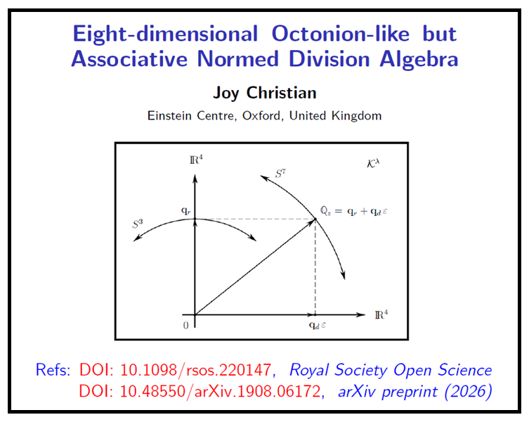
It turns out that this local-realistic framework can be generalized to reproduce ALL quantum correlations, provided we take the codomain of the above functions to be an absolutely parallelized 7-sphere instead of a 3-sphere:

$\displaystyle \pm\,1\,=\,{\cal A}({\bf a},\,\lambda):{\rm I\!R}^3\!\times\Lambda\longrightarrow S^7\hookrightarrow{\rm I\!R}^8. \ \ \ \ \ \ \ (4)$

In fact the choice of $S^7$ here is both necessary and sufficient to provide a complete local account of ALL quantum correlations. It may seem ad hoc, but it stems from the profound relationship between the normed division algebras and the parallelizability of the unit spheres. As is well known, the only spheres that can be parallelized absolutely are ${{S^0}}$ , ${{S^1}}$ , ${{S^3}}$ , and ${{S^7}}$ , and they correspond precisely to the four division algebras: ${{\mathbb R}}$ , ${{\mathbb C}}$ , ${{\mathbb H}}$ , and ${{\mathbb O}}$ . The 7-sphere is thus homeomorphic to the set of all unit octonions, and corresponds to the most general possible normed division algebra ${{\mathbb O}}$ . It is therefore fitting that it also gives rise to the existence and strength of ALL quantum correlations. That is to say, quantum correlations exist and exhibit the strength they exhibit because the equality

$\displaystyle (x_1^2 + x_2^2 + \dots + x_n^2)\,(y_1^2 + y_2^2 + \dots + y_n^2) \,=\, z_1^2 + z_2^2 + \dots + z_n^2 \ \ \ \ \ \ \ (5)$

holds only for the integers ${{n = 1,\;2,\;4}}$ , and ${{8}}$ , for any generalized numbers x. Among the four parallelizable spheres, however, only ${{S^3}}$ and ${{S^7}}$ are non-trivially parallelized, and thus characterized by a non-vanishing torsion. Therefore, only with the choices ${{S^3}}$ and ${{S^7}}$ for the codomain of the measurement functions (4) can we reproduce the strong quantum correlations. Moreover, ${{S^7}}$ can be viewed as a 4-sphere worth of 3-spheres in the language of Hopf fibration (cf. this page). Thus, in general, we only need to consider ${{S^7}}$ , since ${{S^3}}$ is already contained within it as one of its fibres.

This last observation suggestes that for general quantum correlaions the form of the measurement functions (4) has to be generalized to admit an interpediate stage (or map) by giving it the form

$\displaystyle \pm\,1\,=\,{\cal A}({\bf a},\,\lambda):{\rm I\!R}^3\!\times\Lambda\longrightarrow {\rm I\!R}^7\!\times\Lambda\longrightarrow S^7\hookrightarrow{\rm I\!R}^8, \ \ \ \ \ \ \ (6)$

where ${\rm I\!R}^7$ is a tangent space at a point of $S^7$ , spanned by vectors of the form ${\mathbf N}({\mathbf a})$ , with ${\mathbf N}\in{\rm I\!R}^7$ and ${\mathbf a}\in{\rm I\!R}^3$ (explicit constructions of how this map works in practice can be found in this paper). Thus, although the actual measurement results $\pm\,1$ are occurring in the familiar 3D tangent space ${\rm I\!R}^3$ of $S^3$ , their observed values are dictated by the trivial tangent bundle structure ${\rm T}S^7\!=S^7\times{\rm I\!R}^7$ of the absolutely parallelized 7-sphere. In this sense, then, quantum correlations are the evidence of the fact that rotational symmetries respected by our physical space are those of a parallelized 7-sphere. It is important to note here, however, that, unlike the torsion within $S^3$ , the non-associativity of the octonionic numbers leads to torsion within $S^7$ that is necessarily different at each point p of $S^7$ :

$S^3\ni{\cal T}_{\,{\bf a\,a'}}({\lambda}) \xrightarrow{\;S^3\longrightarrow\,S^7\;}{\cal T}_{\,{\bf N(a)\,N(a')}}(p,\,{\lambda})\in S^7. \ \ \ \ \ \ \ (7)$

This variability of torsion gives rise to the rich variety of quantum correlations we observe in nature.

Suppose now we consider an arbitrary quantum state ${|\Psi\rangle}$ and a corresponding self-adjoint operator ${\cal\widehat O}({\bf a},\,{\bf b},\,{\bf c},\,{\bf d},\,\dots\,)$ in some Hilbert space ${\cal H}$ , parameterized by an arbitrary number of local contexts ${{{\bf a},\,{\bf b},\,{\bf c},\,{\bf d},}}$ etc. Note that I have imposed no restrictions on the state ${|\Psi\rangle}$ , or on the size of the Hilbert space ${\cal H}$ . In particular, ${|\Psi\rangle}$ can be as entangled or unentangled as one may like, and ${\cal H}$ can be as large or small as one may like. The quantum mechanical expectation value of the operator ${\cal\widehat O}({\bf a},\,{\bf b},\,{\bf c},\,{\bf d},\,\dots\,)$ in the state ${|\Psi\rangle}$ would then be

$\displaystyle {\cal E}_{{\!}_{Q.M.}}({\bf a},\,{\bf b},\,{\bf c},\,{\bf d},\,\dots\,)\, =\,\text{Tr}\left\{{W}\,{\cal\widehat O}({\bf a},\,{\bf b},\,{\bf c},\,{\bf d},\,\dots\,)\right\}, \ \ \ \ \ \ \ (8)$

where ${{W}}$ is a statistical operator of unit trace representing the state. As noted, I have imposed no restrictions whatsoever on the state, the observable, or the number of local contexts. Nevertheless, it turns out that—because the octonionic division algebra remains closed under multiplication—the quantum correlation predicted by this expectation value can always be reproduced as local and realistic correlation among a set of points of a parallelized 7-sphere, by following a procedure very similar to the one discussed on the previous page. This leads us to the following awesome theorem:

Every quantum mechanical correlation can be understood as a deterministic, local-realistic correlation among a set of points of a parallelized 7-sphere, specified by maps of the form

$\displaystyle \pm\,1\,=\,{\cal A} ({\bf a},\,\lambda): {\rm I\!R}^3\!\times\Lambda\longrightarrow {\rm I\!R}^7\!\times\Lambda\longrightarrow S^7 \hookrightarrow{\rm I\!R}^8. \ \ \ \ \ \ \ (9)$

The proof of this theorem can be found in this paper as well as on the pages 13-17 of my book.

The Raison D’être of Quantum Correlations:

The above theorem demonstrates that the discipline of absolute parallelization in the manifold $S^7$ of all possible measurement results is responsible for the existence and strength of all ${{\,}}$ quantum correlations. More precisely, it identifies quantum correlations as evidence that the physical space we live in respects the symmetries and topologies of a parallelized 7-sphere. There are profound mathematical and conceptual reasons why the topology of the 7-sphere plays such a significant role in the manifestation of quantum correlations. Essentially it is because 7-sphere happens to be homeomorphic to the most general possible division algebra. And it is the property of division that turns out to be responsible for maintaining strict local causality in the world we live in.

To understand this reasoning better, recall that, just as a parallelized 3-sphere is a 2-sphere worth of 1-spheres but with a twist in the manifold ${{S^3\;(\not=S^2\times S^1)}}$ , a parallelized 7-sphere is a 4-sphere worth of 3-spheres but with a twist in the manifold ${{S^7\;(\not=S^4\times S^3)}}$ . More precisely, just as ${{S^3}}$ is a nontrivial fiber bundle over ${{S^2}}$ with Clifford parallels ${{S^1}}$ as its linked fibers, ${{S^7}}$ is also a nontrivial fiber bundle, but over ${{S^4}}$ , and with entire 3-dimensional spheres ${{S^3}}$ as its linked fibers. Now it is the twist in the bundle ${{S^3}}$ that forces one to forgo the commutativity of complex numbers (corresponding to the circles ${{S^1}}$ ) in favor of the non-commutativity of quaternions. In other words, a 3-sphere is not parallelizable by the commuting complex numbers but only by the non-commuting quaternions. And it is this non-commutativity that gives rise to the non-vanishing of the torsion in our physical space. In a similar vein, the twist in the bundle ${{S^7\not=S^4\times S^3}}$ forces one to forgo the associativity of quaternions (corresponding to the fibers ${{S^3}}$ ) in favor of the non-associativity of octonions. In other words, a 7-sphere is not parallelizable by the associative quaternions but only by the non-associative octonions. And the reason why it can be parallelized at all is because its tangent bundle happens to be trivial:

$\displaystyle {\rm T}S^7\,=\!\bigcup_{\,p\,\in\, S^7}\{p\}\times T_pS^7\,\equiv\,S^7\times{\rm I\!R}^7. \ \ \ \ \ \ \ (10)$

Once parallelized by a set of unit octonions, both the 7-sphere and each of its 3-spherical fibers remain closed under multiplication. This, in turn, means that the factorizability or locality condition of Bell is automatically satisfied within a parallelized 7-sphere. The lack of associativity of octonions, however, entails that, unlike the unit 3-sphere [which is homeomorphic to the spinor group SU(2)], a 7-sphere is not a group manifold, but forms only a quasi-group. As a result, the torsion within the 7-sphere continuously varies from one point to another of the manifold. It is this variability of the parallelizing torsion within ${{S^7}}$ that is ultimately responsible for the diversity and non-linearity of the quantum correlations we observe in nature:

$\text{\small Parallelizing Torsion}\;\,{\cal T}_{\,\alpha\,\beta}^{\,\gamma}\not=0\;\;\;\Longleftrightarrow\;\;\;\text{\small Quantum Correlations.}$

The upper bound on all possible quantum correlations is thus set by the maximum of possible torsion within the 7-sphere:

$\text{\small Maximum of Torsion}\;\,{\cal T}_{\,\alpha\,\beta}^{\,\gamma}\not=0\;\;\;\Longrightarrow\;\;\,\text{\small The Upper Bound}\;\,2\sqrt{2}.$

This reaffirms that quantum correlations are a measure of torsion within our physical space.

Home page

49 Responses to Origins of Quantum Correlations

Sandra says:

February 3, 2024 at 11:40 am

Dear Joy,
I’ve spent the last couple of weeks reading about your work. I definitely find it intriguing, but I’m still not understanding some technical details; I just want to ask here about one particular problem that has been bugging me.

In the papers “Restoring Local Causality and Objective Reality to the Entangled Photons” and “Failure of Bell’s Theorem and the Local Causality of the Entangled Photons” (which look to me fundamentally arguing the same things) you use the expression A (α, µ) = (− I · ã ) ( + µ · ã ). The definition of ã is not consistent within the two papers, in one it is ã=ex cos 2α + ey sin 2α while in the other it is defined as ã=ex sin 2α + ey cos 2α.

I’m having a really hard time understanding where these definitions for ã come from; it looks like an ad hoc expression to be able to obtain cos 2(α − β) in the final limit, and is not further justified in the paper. Normally, a refers to the polarization direction chosen by Alice lying in the exey plane at the angle α from ez; it can be expressed as excosα + eysinα in vector form. What does ã stand for, and how has it been derived?

All the best,
Sandra
Joy Christian says:

February 3, 2024 at 1:17 pm

Hi Sandra,

Thank you for your interest in my work and for putting in the effort to understand it.

The reason for the difference in the definitions of ã in the two papers is because of the different polarization states used in them — see equation (15) in both papers. The quantum state (15) used in the paper “Failure …” is EVEN under reflections whereas the quantum state (15) used in the paper “Restoring …” is ODD under reflections. Since the goal of the papers is to reproduce the correlations predicted by these quantum states, it is necessary to parameterize the 2-sphere differently without changing the requirements set by Bell for the definitions of the measurement functions A (α, µ) = (− I · ã ) ( + µ · ã ). In other words, we are free to parameterize the 2-sphere differently using different definitions of the vector ã as long as the polarization angle α is not affected and can be freely chosen by Alice to make her measurements. Note that the result A (α, µ) = +/-1 on the left-hand side of the above equation is not affected by the different definitions of ã. And that is all that matters to satisfy the requirements set by Bell.

I hope this explanation helps.

All the best,
Joy
Sandra says:

February 3, 2024 at 3:51 pm

Thank you Joy for the fast reply. I understand now the reason for the difference, but it’s still nebulous to me the physical significance of ã. Had we used any other parametrization we would not have obtained the right correlation between measurements. But in actual experiments all we can choose are the angles α and β. What physically prevents us to use a different parametrization? My question might have an obvious answer, I’m just not yet familiar with the intricacies of geometric algebra.
Joy Christian says:

February 3, 2024 at 4:45 pm

The question here is not about geometric algebra but about (1) what freedom Bell’s theorem allows us in the definition of the measurement function A (α, µ) = +/-1, and (2) how the coordinates are set up by the experimentalists in the Bell-test experiments involving photons?

The answer to the first question is that Bell’s theorem allows us *complete* freedom in the definition of measurement functions. Bell says that we can choose whatever functions we like, however complicated (or simple) we like. The only requirement he sets is that the left-hand side of the functions must depend *only* on the hidden variable µ and the chosen experimental setting α, nothing else. Thus you are needlessly worried about the specific choice of the expression I have made on the right-hand side in defining A (α, µ) = (− I · ã ) ( + µ · ã ).

But you may ask: Why have I made that particular choice? The answer is: To match with the coordinates and settings used by the experimenters in those specific experiments. If you make a different choice for ã, for example, then you would still be able to derive the cosine correlations, but they may not match with the settings α. You may end up with something like -cos(a, b), where a and b vectors would be your new choice of vectors. Then, for you, the task would be to match with the coordinates used by the experimentalists. You would then end up with my choice for ã.
Sandra says:

February 3, 2024 at 9:46 pm

Thank you very much again Joy. It’s a great feeling when researchers are so easily available for the general public questions. In case I have more doubts that I don’t find easily answered in your other reply papers, would it bother you if I were to ask away? Would this blog be appropriate, or would you rather other online addresses? In any case, good luck with your research program. Even if it doesn’t turn out to be the right path forward, we need new ideas like yours.

Sandra

PS: I also read “Completing the Theory of Electron with Gravitational Torsion”. I’m not sure whether it might be of any interest to you, but I once read some interesting (albeit VERY speculative) ideas about the electron structure. You might want to check “Is the electron a photon with Toroidal Topology?” by Williamson and Van der Mark. Maybe not quite toroidal, maybe more like an Hopf fibration.
Joy Christian says:

February 3, 2024 at 11:00 pm

You are welcome, Sandra. I will be happy to answer any reasonable questions. This blog is a good place for discussion. That way other people may also benefit from your questions.
Sandra says:

February 5, 2024 at 3:06 pm

Hi again. It wasn’t too long until I found some other thing that escapes my comprehension.
In the original one page paper “Disproof of Bell’s Theorem” and subsequent more in-depth “On the Origins of Quantum Correlations”, you differentiate between raw and standard scores. It is my understanding that these correspond respectively to actual measured values (i.e. the detector outputs, as a raw score) and the true value of the measurement (the standard score). Is this a correct intepretation? You reason this differentiation is necessary because the two measurements have different standard deviations, and this is because each score “depends
on different units and scales (or different scales of dispersion) that
may have been used (advertently or inadvertently) in the measurements of such scores.” Why is that? Is it because for each measurement the detector bivector D(n) is different?
In a more recent paper (“Bell’s Theorem Versus Local Realism in a Quaternionic
Model of Physical Space”) you calculate the correlation function using the quaternionic spin values s1 and s2 instead. This paper makes no mention of standard deviations. Is this because the derivation here corresponds to using the “true value” of the measurement, i.e. the standard score, automatically?
Joy Christian says:

February 6, 2024 at 5:42 pm

Thank you, Sandra, for further questions.

There are several different ways to compute correlations within S^3. In the original one-page paper, correlations are computed using Pearson’s correlation coefficient, albeit applied to bivectors within geometric algebra. You can find Pearson’s method in this Wikipedia page:

https://en.wikipedia.org/wiki/Pearson_correlation_coefficient

This method, applied within S^3, is explained in more detail after Eq. (104) in this paper:

https://arxiv.org/abs/1211.0784

In your post above, you have understood my reasoning correctly.

In the recent paper published in IEEE Access, on the other hand, the correlations are computed using the phenomenological method used by the experimentalists. This method, as you note, involves the standard scores automatically, by construction.

Theoretically, both methods are equivalent and give the same results for the correlations.
Sandra says:

April 4, 2024 at 3:32 pm

Hi again Joy.
So, after a bit more reading I came to the paper “Dr. Bertlmann’s Socks in the Quaternionic World of Ambidextral Reality”. I really liked this paper because it shows a very clear example in 2D of the basic idea. Still, I recognize that this example is not exactly a perfect analogy for the 3-sphere case. In particular, I find it hard to picture what exactly it means for our physical space to be “parallelized”, or having the topology of a 3-sphere in the first place. I was always taught that the overall intrinsic curvature of the universe reflects on parallel rays staying parallel or not as they travel, or alternatively about the angles of a big enough “triangle” exceeding 180°. The entanglement results are supposed to be caused by the topology of our space, but these are performed locally, how can the curvature, which locally is indistinguishable from flat, have any effect?

Another thing that escapes my intuition is about the Hopf fibration, and how it relates to the physical experiments. I understand how, in the words of Eric Weinstein, the map S3 to S2 effectively corresponds to little circles at each point in spacetime. These circles (their angle, 2π), in your paper, are assigned to the angle formed by the measurement vector (a or b), which is decided by Alice and Bob, and the spin bivector s. In this sense I’m picturing that each point on the sphere effectively has a phase attached to it, going from 0 to 2pi. Then, the angle between a and b is assigned to the equatorial angle of the sphere. I’m failing to picture how in my mind the “phase” cycles at each point as the equatorial angle goes from 0 (where the 2 phases, or Hopf fibers, are identical) to π (where they get a – sign), and how physically this happens as I rotate the detectors/polarizers. I’m also failing to understand what the vertical angle stands for: for the equatorial angle 0, all the points between 0<rho<π are supposed to have the same twist in the fiber; their projections though are obviously different, being larger and larger circles as rho gets smaller.

On another note, have you thought about appearing on famous physics podcasts like Brian Keating's or Kurt Jomungal? The latter I think would be delighted to have you. This would help a lot getting your ideas out there.
Joy Christian says:

April 5, 2024 at 9:25 am

Hi Sandra,

The concept of parallelizability of space (or manifold) has nothing to do with Euclid’s parallel postulate, or parallel rays, or triangles exceeding 180°. It has to do with the possibility of assigning a consistent sense of handedness throughout the space. The toy example of the 2D Mobius strip is a good counter-example of this. On a Mobius strip, we cannot consistently assign handedness throughout the space. Because of the twist in the space, the handedness changes from left to right or right to left as we go around the strip. By contrast, on the 3-sphere the quaternions that constitute it assign a consistent sense of orientation or handedness throughout the sphere, without exception — i.e., without a single point left out to have a different handedness from the rest of the points. In the technical language, this means that a 3-sphere is parallelizable. And the very quaternions that constitute the 3-sphere, parallelize it.

I am afraid it is not easy to develop intuition about the geometry of the 3-sphere. Your understanding of the Hopf fibration, namely, that a circle, S1, is attached to each point of the base space S2, is correct. However, it is not easy to visualize how the phase angle of each quaternion “conspires” to produce the strong correlations we observe in the experiments. Unlike in the 2D example of the Mobius strip, for the 3-sphere it is necessary to follow the mathematics of the quaternions to understand what is going on. In this regard, perhaps my latest paper may help, because in it I work out the mathematics in more detail. See, especially, Section V of the paper:

https://arxiv.org/pdf/2204.10288.pdf

Some months ago Kurt Jomungal had approached me about appearing on his podcast to explain my model. But then he lost interest for some reason. I guess he found my model too difficult or too controversial for his podcast.
Sandra says:

April 6, 2024 at 2:42 pm

Thank you for your answer Joy.
I have used this online tool (https://philogb.github.io/page/hopf/#) to visualize 2pi rotations of a fibration. Indeed, the motion of the circle is such that any point on the fibration will find itself 180 degrees from its starting position, after a 2pi rotation on S2.
.
I’m still not sure how detectors can differentiate between the two signs: might it be that it’s because they use Stern-Gerlach apparatuses? The relationships in the electromagnetic field behave eerily similar to quaternion rotations, like the current in a wire generating a magnetic field with the right hand rule. So basically we’re testing handedness with another intrinsically chiral apparatus.
.
I find your math completely correct (it’s much easier to follow with L(s) instead of lambda). What I struggle with is what it all means. Spinors are not that hard to visualize if you use belts or rocks attached to ropes. But we’re talking about electrons here; they aren’t belts nor rocks with ropes. It’s clear that there is something rotating about. Could it be space itself? I can visualize a grid moving like in this picture (https://commons.wikimedia.org/w/index.php?title=Special:ListFiles/JasonHise&ilshowall=1#/media/File:Anti-Twister.gif). After all, the only way to continuosly rotate a 3D elastic medium without breaking it (or without the elastic tension going to infinity) is exactly the spinorial motion. Would you agree?
.
It’s unfortunate Kurt never got through with interviewing you. People on the net immediately dismiss your work because they heard some “authorities” like Aaronson or because someone (cough Gill cough) said you violated some Hurwitz theorem, while it’s clear to me that you adressed those criticism perfectly well. In any case, you have my support!
.
PS: did you ever manage to perform the experiment with the exploding balls? It doesn’t sound that expensive. But again, I’m not an experimentalist.
Joy Christian says:

April 7, 2024 at 6:19 am

Thank you, Sandra, for your support and interest in my work. As you can see, considerable effort is required to understand the 3-sphere model based on quaternions. So, thank you for investing your time to try to understand it.

The detectors in the 3-sphere model are modeled by bivectors D(a) and D(b). These bivectors are the counterparts of the vectors `a’ and `b’ used by Bell in his local model within R^3. The actual experiments indeed use Stern-Gerlach apparatuses to detect spins. But in a theoretical model like Bell’s, only the directions of the Stern-Gerlach apparatuses are relevant. In the 3-sphere model, the vectors `a’ and `b’ translate to bivectors D(a) and D(b). The handedness of these detector bivectors is fixed by Alice and Bob for the course of their experiment. The spin bivectors, L(s1) and L(s2) emerging from the source, whose handedness is random (i.e., not fixed by Nature), then interact with the detectors D(a) and D(b), respectively. The mathematics of bivectors then dictates that the resulting values of the spins will be either +1 or -1, as required by Bell and the Bell-test experiments. So, yes, we are measuring the spin handedness with an intrinsically chiral apparatus, because that is precisely the nature of the 3-sphere geometry.

Note also that, as with the belt or rock example, electors in a singlet state are not isolated. They come in pairs. And even though their spins are detected at spacelike separation, the electrons are correlated with each other. However, there is nothing non-local about this correlation. It is like a correlation between a pair of gloves. If you find only one glove in your pocket and it is right-handed, then you instantly know that the one you forgot at home is left-handed. In other words, the two gloves are correlated. It is the same with a pair of electrons in a singlet state. But that correlation also means that the electrons are rotating with respect to each other. So, the “belt” in this case is the preexisting correlation between the electrons, like that between the glove in your pocket and the one you forgot at home. More locally, the spinning electron L(s) is spinning with respect to the detector D(a) of fixed-handedness. Thus, the situation here is no different from that with a belt or a rock. It is just that a “belt” in this case is more abstract.

The experiment you mention would indeed be rather inexpensive. However, I am also not an experimentalist, so I can’t perform the experiment myself. Besides, it must be performed independently by some well-known experimentalists for the community to take the results seriously. Unfortunately, the negative propaganda about my work by the non-physicists you mention has so far prevented any serious experimentalists from taking an interest in my work or my proposed experiment.
Sandra says:

April 10, 2024 at 4:38 pm

Another thing I’m not sure I understand, that you might have already clarified in some other paper. In the paper you last linked me “Symmetric derivation of singlet correlations in a quaternionic 3-sphere model”, you say:

− L(s1) + L(s2) = 0 ⇐⇒ L(s1) = L(s2)
⇐⇒ s1 = s2 ≡ s.

Because of conservation of angular momentum. You use this notation in other papers as well, but shouldn’t it be L(s1) + L(s2) = 0 ⇐⇒ L(s1) = – L(s2) ? S is the spin direction, and it makes sense for both particles to have the same direction, but shouldn’t it be of opposite sign? I might be getting confused here.
.
Later in the paper you define the measurement functions
.
S3 ∋ A (a, si1) = lim s1 → µ1a {− D(a)L(s1)}
and
S3 ∋ B(b, si2) = lim s2 → µ2b {+ L(s2) D(b)}
.
I don’t quite understand why the two have a different sign inside the parenthesis. It was established L(s1) = L(s2) so the sign can’t come from L(s). D(a) and D(b) are freely chosen bivectors.
Joy Christian says:

April 10, 2024 at 8:57 pm

This one is easy to sort out. The sign convention for spins is chosen to respect the fact that unit bivectors square to -1 in Geometric Algebra. As shown in Figure 1 of the “Symmetric” paper you mention, the two spins are rotating in the opposite senses of each other, but about the same vector s1 = s2 = s. Now, instead of what I have chosen in the paper, let us set L(s1) + L (s2) = 0 as you have written. Then we indeed have L(s1) = -L(s2), as you say. But then the product of the two spins will give -L(s)L(s) = -(I s)(I s) = +1, because the squared bivector (I s)^2 = -1 in Geometric Algebra. Here `I’ is the standard trivector. Thus, the square of the two spin momenta gives the wrong sign. I have preferred the sign convention for spins to be consistent with the standard use of minus sign for the square of the unit bivectors in Geometric Algebra.

The signs in the definitions of the measurement functions also come from how I have defined the spins for Alice and Bob. I have denoted the spin approaching Alice’s detector D(a) to be -L(s1), and the spin approaching Bob’s detector D(b) to be +L(s2). That is where the signs in the measurement functions come from. Also, the functions A and B must be chosen so that for the perfect correlation, i.e., when a = b, the product A(a)B(a) must be equal to -1. This requirement comes from the definition of the singlet state as well as the original EPR-Bohm argument. If we drop the sign difference from the measurement functions then the requirement A(a)B(a) = -1 is not respected.
Sandra says:

April 11, 2024 at 12:12 am

Thank you again Joy. Yes that sorted it out, it makes sense: the sign is purely a convention, and here it’s preferable to make it explicit.
.
It’s wild to me your work is getting ignored like this. You know, this journey for me started around 2 years ago when I posted on a physics forum a question about bell’s theorem and how it looked like we were missing something about the detectors themselves. I still didn’t quite have clear the whole issue, but I got surprisingly close (detectors are bivectors!). I also mentioned that it did not make sense to use counterfactuals to derive the inequality. I was met with extreme dismissal, the thread was locked before I could reply, and subsequent posts with questions on unrelated things had as first answers something like “oh you’re the nut that posted about bell’s theorem this is going to be long” . I’m usually very self aware about what I think I know; especially in physics, whenever there is some talk about very complicated stuff like gauge theory, QCD, yang-mills, symmetry breaking… I always tell myself “it’s not so easy. You’re missing so much before you can even comment on these things”.
.
But when I look at your work, I can follow it. It is logically sound. I look around for criticisms, because I remind myself “it can’t be so easy!”, but all I see are people completely missing the point. The SAME people that do complicated stuff like gauge theory, yang-mills, etc. are missing the point. It’s disorienting. I’m feeling pretty confident you are right, yet I can’t shake this uncertainty about everything else. The best hidden things are those right under our noses I guess.
.
Sorry for rant, and thank you again Joy.
Joy Christian says:

April 11, 2024 at 8:46 am

You are welcome, Sandra.

Yes, the reaction of some members of the community to my work is surprising. It seems that Bell’s theorem has become a kind of religion for some people. They get offended if you tell them that it is based on mistaken assumptions and that you can demonstrate that. Instead of people showing interest in my work, I have encountered much abuse, knee-jerk reactions, and ostracization from some members of the Bell community. But slowly some people in the community (like yourself) have begun to take a positive interest in my work. So there is hope that, eventually, people will understand what I have been saying.
Sandra says:

May 18, 2024 at 4:17 pm

Hi Joy,
I have a question concerning the relationship between the validity of additivity of expectation values and fine’s theorem, which states (unless i misunderstood) that all bell theorem says is that there are no joint probability distributions for non commuting observables.
.
Are these two statements equivalent?
.
Does additivity of e.v. imply existence of a joint probability distribution and vice-versa? Or are these completely unrelated? My confusion possibly arises because I didn’t quite get what it means to have a joint probability distribution. Maybe you can give me a simple example involving three simultaneous coin tosses with heads or tails. I’m struggling to see why we can’t define at least counterfactually some probability distribution for the three coins results, even though we are able to toss only two coins.
.
Also, is it correct to say that additivity of e.v. is not respected because what we average over in non-commuting observables are not real quantities (i.e. don’t fit on the real line of numbers)? Like in the case of spin, we’re averaging over limiting scalar points of quaternions. Bell’s inequality assumes spins are vectors, which can be put into a 1:1 correspondence with the real line.
.
Thank you for taking time to address my questions.
Joy Christian says:

May 18, 2024 at 9:18 pm

Hi Sandra,
Fine’s theorem does not say what you say it does. But I know what you are talking about. It says that CHSH inequalities are not only necessary but also sufficient conditions for the probabilities of the pairs of joint measurement results (thought of as pairs of random variables) to be the marginals of the probability of all four random variables involved in the Bell-test experiments. This theorem is not disputed by anyone, as far as I know.

However, Fine has also argued that the assumption of joint probability distributions for non-commuting observables is unreasonable. But if regarded as random variables in a hidden variable theory, all observables, whether commuting or not, have well-defined joint probability distributions. Therefore, Fine’s objection is not accepted by the proponents of Bell’s theorem.

The issue I have raised about the non-additivity of expectation values for hidden variable theories is much more serious. Although related, it is not equivalent to the issue of the existence of a joint probability space for all four pairs of random variables. In particular, the additivity of expectation values implies the existence of a joint probability space, but not vice versa.

There is no problem with either issue in your example of three simultaneous coin tosses because in that case no non-commuting observables are involved. Therefore, for that example, we can indeed define a joint probability space without difficulty.

By contrast, the additivity of expectation values is not respected for non-commuting observables involved in the Bell-test experiments because their values are not sharply defined. For example, the uncertainty principle dictates that if the position of a free particle is sharply defined then its momentum is not, and vice versa. So, indeed, the possible values of both position and momentum cannot be simultaneously assigned numbers on a real line. In a hidden variable theory, values of observables are eigenvalues of the corresponding quantum mechanical operators, and eigenvalues do not add linearly for non-commuting observables. Consequently, the expectation values do not add linearly either.
Sandra says:

May 19, 2024 at 8:00 am

Thank you Joy. Indeed I was a bit confused about fine’s argument.
.
I brought up the coins because it is a popular way to derive Bell’s inequality P(A, notB) + P(B, not C) >= P(A, not C). It was indeed my suspicion that here bell comes out right simply because the coins do no represent non-commuting quantities. So basically this derivation is completely irrelevant to bell tests.
.
You say “For example, the uncertainty principle dictates that if the position of a free particle is sharply defined then its momentum is not, and vice versa. So, indeed, the possible values of both position and momentum cannot be simultaneously assigned numbers on a real line.” Isn’t that the point of hidden variables though? That there actually is a value for both at the same time, but hidden from us due to the nature of measurement? I’m struggling a little bit here: you derived Bell correlations by assuming the spin is actually pre-defined, as a bivector.
Joy Christian says:

May 19, 2024 at 8:52 am

Yes, the derivations of Bell inequalities are completely irrelevant to the Bell-test experiments, which inevitably involve non-commuting observables.

And, yes, it is indeed the point of hidden variables that there actually are sharp values for both position and momentum at the same time, which are hidden from us because of our inability to measure them simultaneously. But these sharp values cannot be any old sharp values even in a hidden variable theory. They have to be specific eigenvalues of the corresponding quantum mechanical operators. This is the fundamental difference between classical theory and a hidden variable theory. Hidden variable theories are not classical theories. They have to reproduce the precise statistical averages predicted by quantum mechanics. And that can be done only by averaging over specific eigenvalues of the corresponding quantum mechanical operators. The mistake in Bell’s argument is thus the assumption that the sharp values of observables like position and momentum add linearly. But sharp values as specific eigenvalues of the corresponding operators do not add linearly.
Sandra says:

May 30, 2024 at 9:34 pm

I took a bit of time to think about your last answer. Is it related to the whole “one point of the sphere represents a point at infinity of the plane R2″ business? For example, if we represent spin as a vector spanning the sphere, the measurement result (the application of a particular operator) will be the projection of the tip of the vector onto the plane defined by the measurement direction choice. But for at least one vector (one pointing at the north pole and perpendicular to the plane) there is no clearly defined projection, since it represents a point at infinity in all directions. To define the measurement of THAT vector, we need a different operator. But in any case, none of this means that the vector itself is indefinite, only our measurement of it with respect to a particular plane (operator) is. Since the plane is made of real numbers, any such vector cannot be described as a real number. Am i in the right direction? I think i’m missing the step of how we go from this picture to S3. Are we simply changing the nature of the projective plane? Are we “wrapping a sphere” around that spanned by the spin vectors and projecting on to it? I’m aware spinors are not vectors but bivectors. I’m just trying to glue it all together and im still digesting you paper about the octonion-like division algebra.
Joy Christian says:

May 31, 2024 at 8:47 am

I think it is best not to focus on the octonion-like paper before understanding why S^3 is needed. You are right to try to understand the move from the usual S^2 picture with ordinary vectors to S^3 and bivectors (i.e., pure quaternions). But the octonion-like paper is not best for this. It is more involved and concerned with a larger goal of involving S^7, which is a more complicated space. So, let us first focus on S^3, which is discussed in the following paper, for example, which you have already seen as a preprint:

https://doi.org/10.1007/s10773-024-05639-2

The point at infinity business is only indirectly connected to the problem at hand, which is to understand how the strong correlations observed in the Bell-test experiments arise naturally if the physical space is modeled as S^3 instead of R^3. Topologically, moving from R^3 to S^3 has to do with the point at infinity, but that is just the beginning. Once we arrive at S^3, we recognize that it is best represented by the set of unit quaternions, for various topological and geometrical reasons. Now quaternions and bivectors (the latter being “pure” quaternions, i.e., without the scalar parts) are naturally non-commutative. Moreover, this non-commutativity is free of all the quantum mechanical baggage like operators and projections postulate to extract observed results from the operators. They are non-commutative for purely geometrical reasons, not quantum mechanical reasons. So, we have a happy situation in S^3 in which we can have our cake and eat it too. Namely, we can have non-commutativity, which is responsible for producing strong quantum correlations, but without the unwanted features like non-locality or non-reality.

But what about the point at infinity, you may ask? Well, it is best to leave it behind. It was just a means to an end. The end goal was to understand the strong correlations in a satisfactory way in terms of quaternions and bivectors constituting S^3, and we have done that.
Sandra says:

May 31, 2024 at 10:55 am

Ok, so the basic idea is S3 is there to remove us from the quantum mechanical formalism which is limiting, and instead of completing quantum mechanical states with a contextual hidden variables we simply change the formalism and instead use the relationship between points, lines, surfaces and volume elements of geometric algebra, where instead of projections and operators to represent measurements we have simple multiplication between points of S3. But can all physical quantities be represented as points on S3? I see how this is easy for spinors since these are naturally pure quaternions, (and also for stern Gerlach magnets) but what about position or momentum? Position seems like a scalar quantity, while momentum… I’m not really sure, but it looks like another scalar number. What about time and energy, which also seem both scalars?
Sorry if I’m bombarding you with question and perhaps misconceptions. I know your math is right, and I understood how the correlations arise because of S3, but I am way more of a visual person and to really understand something I need a mental picture of how it all fits together.
Joy Christian says:

May 31, 2024 at 11:52 am

Intuitions and mental pictures can be developed about all this, but that takes time. Unfortunately, mental pictures can also be misleading. So, we must be careful about them and follow the math as much as possible.

Your question now is about all possible observables, including continuous observables such as position and momentum. As we know, in quantum mechanics all observables and states of physical systems are represented by Hermitian operators in Hilbert space. Can they also be represented by points of S^3? No, that is not possible. S^3 is too small a space for that. That is why S^7 is needed, as I have explained in the Octonion-like paper. It turns out that the S^7 needed for this purpose is an algebraic representation space of the quaternionic S^3. So, it is also a Clifford-algebraic space.

Now, to represent all observables we have to go back 92 years and study what von Neumann taught us about how to construct a hidden variable theory for all observables (see his book on QM published in 1932). The trick is to reduce all experimental questions into questions with only “yes” or “no” answers. Such binary questions can then be represented as projection operators in Hilbert space, with eigenvalues, say +1 for “yes” and -1 for “no.” For example, for the position observable X of an electron, we can reduce the problem with questions like: “Is the electron located at x = 3 c.m.?” If the answer is “yes”, then we have only the eigenvalue +1 to worry about, and if the answer is “no” then we have only the eigenvalue -1 to worry about, even though the position of an electron is a continuous variable.

O.k., that is within quantum mechanics. But now you can see that I can use the scalar points of S^7, just like those of S^3, to represent the binary eigenvalues +1 and -1 for any observables. Even continuous observables like position and momentum can be reduced to a set of projection operators within quantum mechanics and scalar points, +1 or -1, within S^7.

Remember that the goal of a hidden variable theory is not to construct an efficient practical theory, which we already have, namely quantum mechanics, but to provide a local-realistic understanding of that practical theory, as Einstein wanted. And the scheme I described above and presented in full detail in the Octonion-like paper does just that.
Sandra says:

June 20, 2024 at 2:37 pm

Hello Joy,
between pauses at work I came back to the detailed calculations in your papers. I looked up wether you already answer this question in the appendix, but couldn’t find anything. In the derivation of the singlet correlations you employ some limit functions, namely for S tending to sign(S*a) and similar for b, to represent the measurement. The derivation for the values +1 or -1 of the measurement for either alice or bob rest on this limit, no problem so far. Then, you use the “product of limits equals the limit of the product” rule, and doing so you’re able to cancel the spin bivectors in the joint measurement since their geometric product =-1 due to conservation of angular momentum. The result is then -cos(ab).
My issue is twofold here: in bell tests, the correlation function is obtained with the values of +1/-1 from single measurements at Alice and bob’s stations; this means that they are using the values obtained for when the spin bivectors were already “gone through” the application of the limit, and as such the new value for the spin at Alice is +a/-a and for bob it is +b/-b. When we perform multiplication between these two spin values L(s)L(s) not equal to -1 anymore, since the conservation of angular momentum can’t apply post-measurement. Second, even if what I just said is not the case, the correlation for a single measurement is not an integer. I know you talk about limiting scalar points, but this in the product quaternion q(ab) would correspond to the angle AB tending to zero; I’m also aware that QM is a statistical theory, but this derivation does not rely on a large number of measurements. So I’m a bit confused here.
There is also a third thing I noticed; your derivation seems to apply just fine if instead of geometric product between quaternions or bivectors we just use the scalar product between vectors. The limit of S tends to sign(S•a) is still +a or -a, so the result at Alice station is still +1/-1. For the correlation AB, we have lim(S•a) • lim(-S•b) = lim [S•a • -S•b]. Since the dot product is commutative, this equals to [S•-S•a•b] = – a•b.
As usual I’m confident you’ll clear up my confusion.
Joy Christian says:

June 20, 2024 at 9:46 pm

Hi Sandra,

You seem to be misinterpreting the computation of the correlations presented in equations (57) to (63) of this paper:

https://link.springer.com/article/10.1007/s10773-024-05639-2

The correlations in these equations are being computed between the numbers A = +/-1 and B = +/-1, just as they are in Bell’s local model and the Bell-test experiments. This is clear from equation (57). The only difference is that in the 3-sphere model the numbers A = +/-1 and B = +/-1 we see in equation (57) are limiting scalar points of the quaternions that constitute the 3-sphere. Therefore, the steps (58) to (63) of the computations must respect the fact that A = +/-1 and B = +/-1 are the points of the 3-sphere, S^3, and not those of R^3. In other words, the steps (58) to (63) are simply mathematical steps that respect the geometry of the 3-sphere. The experiment is long finished. It was finished at step (57). The rest of the steps are merely theoretical calculations. Remember that the 3-sphere model is a theoretical model that predicts the correlations, not an after-the-event experimental procedure followed by the experimenters.

As for your second point, the correlation for a single measurement is an integer, AB = +/-1. You can verify that from equation (29). Note that a 3-sphere remains closed under multiplication. That means a product of two unit quaternions is also a unit quaternion within the 3-sphere. Therefore, AB = +/-1 is also a limiting scalar point within the 3-sphere. If you don’t see that in the steps (58) to (63) of the computation, then that is because of what I explained in the above paragraph.

As for your third point: your mathematics with dot products is all wrong. The sign(s.a) or lim(s.a) are scalar numbers. You cannot take a dot product between two scalar numbers. That is just wrong mathematics. You also cannot move around the dot product as you have done. That is an illegal or meaningless operation. And even if what you are doing were mathematically correct, what would it mean? It is not a computation of the correlations between the scalar numbers A = +/-1 and B = +/-1 as in my equations (57) to (63). What you have done will not give you -a.b if you use correct mathematics.

I hope this helps.
Sandra says:

June 21, 2024 at 9:25 am

I do see your point about the mistake with the dot product, I didn’t think about it. That clears it up.
In your paper you write: “A and B encode local physical interactions taking place during the detection process at the two ends of the experiment. [...] SG devices are knows to align spin directions to their orientations”. I take it then that by “limiting scalar point” you mean this process of alignment. In quaternion terms, this corresponds for example to q(s1-a, r) for when the angle s1-a tends to 0.
So when you derive the correlation product, which is essentially a quaternion product of q(s1-a,r1)q(s2-b,r2) = q(a-b, r), the corresponding limiting scalar would result from the limit as the angle a-b tends to 0. At least, that’s how I interpreted the equations. This is what I meant that gives me confusion.
On an unrelated note, I also noticed that the relationship between these quaternions has an intriguing geometrical picture: in S2, the detector directions represent two equatorial planes; at angle 0, these two planes coincide. When you increase the angle between them it’s like rotating one of these two planes on an axis, say on the x axis. The corresponding product quaternion is another equatorial plane, that is instead rotated on an orthogonal axis, say y, by the same angle. If you shine a light on top of this last plane, as it rotates it forms a shadow underneath (a projection) whose area is exactly cos(alpha), with alpha being the angle difference between the detectors. I don’t know if you are already aware of this picture, and if it actually has some relationship to actual physics here.
Joy Christian says:

June 21, 2024 at 11:34 am

Yes, the limits simply align the spin direction “s” to the detector directions “a” and “b” at the two ends of the experiment.

But the detector directions “a” and “b” are fixed by Alice and Bob. They cannot change throughout a run of the experiment. So, the angle between them also cannot change. Only the spin direction “s” gets aligned to “a” and “b”, respectively, during the detection processes, which are physical interactions taking place within the SG devices. See equation (50) where limits are taken jointly on both sides. Because the detection processes are physical processes external to the spin system, the conservation law L(s1)L(s2) = -1 does not hold during the detection processes. In equation (59), on the other hand, the limits simply drop out from the calculation, so no contradiction occurs even though we have imposed the conservation law.

Yes, the geometrical picture within S2 you describe is intriguing. As you explore further, you will develop a good mental image of the geometries of both S2 and S3 as you hoped to develop in one of your earlier posts.
Sandra says:

July 5, 2024 at 6:06 am

Joy, I think I finally understood what you mean by limiting scalar point. Is it not simply the image we assign to every point of the 3-sphere? The codomain is the “coordinate” of the point (basically, a direction), while the image is a value we assign to that coordinate. This means that multiple coordinates (effectively corresponding to different hidden variables) have the same image. This is what led bell to his mistake: he conflated images with codomain, and in doing so masked the inherent non-commutativity of the true values of the measurement functions, because the images, being real numbers, always commute.
.
But with this reply I actually wanted to ask you something else. What exactly is the difference between an electron and a positron? Is it just the sign of the volume element (or trivector)? How is this related to the handedness of the 3-sphere, are they the same thing? I ask this because I noticed that as solution of the Dirac equation, the only difference between the two spinors is a sign.
Joy Christian says:

July 6, 2024 at 9:31 am

Yes, by “limiting scalar point” I just mean an image within the 3-sphere. In the 3-sphere model, the codomain of the measurement functions, A(a, h) and B(b, h), is the 3-sphere, which is a set of unit quaternions. So, each point of the codomain is a quaternion. But quaternions are not scalars like the functions A(a, h) = +/-1 and B(b, h) = +/-1. So, we must take an appropriate limit of a quaternion to obtain the measurement results +/-1. Mathematically, that limiting scalar point is then an image point within the 3-sphere. In any mathematical function, the set of all possible images is a *subset* of the codomain of that function. In our case, the set of all possible images is thus a set of numbers +/-1, and the corresponding codomain is a set of all unit quaternions, which in turn is just the definition of S^3 or 3-sphere. So, indeed, in Bell’s simplistic model, he conflated the subset of image points (the “limiting scalar points”) with the codomain, “and in doing so masked the inherent non-commutativity of the true values of the measurement functions, because the images, being real numbers, always commute”, just as you say.

Electrons and positrons are both fermions — i.e., spin-1/2 particles. They differ only in their charge. Electrons are negatively charged whereas positrons are positively charged. So, as far as their spinning properties are concerned, there is no difference between them.
Sandra says:

July 6, 2024 at 6:00 pm

I’m pretty sure though that matter and antimatter (not just electrons positrons) are related by a mirror symmetry. After all Charge conjugation is equivalent to Parity and time (momentum) conjugation. I know bivectors are chiral. I was just wondering if the sign of the pseudoscalar, intended as the handedness of the 3-sphere, is connected to the concept of chirality in fermions.
Joy Christian says:

July 6, 2024 at 8:34 pm

The sign of the pseudoscalar may be connected to the concept of chirality in fermions. It can certainly be used for that purpose because changing the sign would change the handedness or orientation of the 3-sphere.
Joy Christian says:

August 31, 2024 at 7:58 pm

I have posted a new short note on arXiv in which I point out a sign mistake in the GHZ variant of Bell’s theorem, invalidating its claim that the premisses of the EPR argument are inconsistent for several particles in an entangled quantum state:

https://doi.org/10.48550/arXiv.2408.10256
Sandra says:

September 2, 2024 at 8:04 pm

Seems like it’s always the same argument, that Bell and co. assumed measurement results are eigenvalues of commuting operators. It’s so simple yet it gets so much resistance.
.
I’ve had some discussions on online forums about this, linked videos and papers, and they all ended up in abuse and even a ban on physicsforums. People seem so convinced Scott Aaronson, Weatherall and so on debunked your model, that they don’t appreciate the fact that none of those “authors” ever even talked about your criticism of Bell, but only and strictly about your 3-sphere model (failing miserably at that…).
.
People don’t want to listen.
Joy Christian says:

September 2, 2024 at 8:56 pm

Yes, it is a very sad situation. I get similar intolerance and abuse from journal editors and peer reviewers — who, unfortunately, have the real power to make or break an idea. It has taken me 17 years to pass only 8 of my papers through the peer review process. Most other papers you see as preprints on arXiv were rejected without ever being sent out by editors for external peer review.

Aaronson’s behavior was quite obnoxious and despicable on his blog some 12 years ago where he attempted to “debunk” the 3-sphere model, without ever bothering to understand what it is.

Weatherall’s paper is the most dishonest paper ever written. It gives the false impression to the reader that he is about to discuss my model but, in fact, he does no such thing. I have refuted his and Aaronson’s claims in the following preprint, which is not on arXiv:
https://zenodo.org/records/6970788
Sandra says:

September 15, 2024 at 2:11 pm

Hi joy, i have to go back talking about your limit function used in “Local origins of quantum correlations rooted in geometric algebra” and other papers, the one with
.
lim(s1 → μ1a) D(a)L(s1)
.
I already asked you a similar question, and you replied that we should think about the product of two such limits giving cos(ab) as a theoretical result, obtained before the after-the-event analysis done in labs.
But the more I keep looking into it, the more i think this result is wonky.
The product of limits equals the limit of product rule is valid if the two limits are the same. But here the two limits are clearly not the same: s1 → μ1a and s2 → μ2b.
Even if we set s1=s2, we can’t multiply the functions inside the limit like -D(a)L(s)L(s)D(b) to get D(a)D(b) BEFORE taking the limit. It’s like saying
.
lim(x->2) x * lim(x->3) 1/x = 2/3
.
but if we first multiply them
.
lim(x->2,x->3) x*1/x = 1
.
this can only be done if the two limits tend to the same value.
This should be noticeable in retrospect because if cos(uv) becomes cos(ab) in the product, this cannot be equal to +1 or -1 unless a = +- b. Yet, in experiments we do the calculations with AB = +-1 even when a is different from b. I hope you understand my concern.
I had been looking for a way to justify the equality of equation 126 of this paper: https://arxiv.org/pdf/2205.11372
Joy Christian says:

September 15, 2024 at 2:57 pm

Hi Sandra,

I will have a closer look at your worry. In the meantime, take a look at the two parallel derivations in this paper published in IJTP, because it has gone through peer review:

https://arxiv.org/abs/2204.10288

First, look at equations (49) to (55), which reproduce the known result derived by Bell in 1964, but using the limits you are worried about.

Then, look at equations (57) to (63), which derive the cosine correlations using the same limits as previously used in (49) to (55). The only difference between the two sets of equations is the use of the conservation law in the second set.

This demonstrates that the use of limits as well as everything else in the two derivations is correct.

Nevertheless, I will take a closer look at the equations in the “Local origins” paper you are worried about.
Joy Christian says:

September 15, 2024 at 6:28 pm

Ok. I have now looked at equation 126 of the “Local origins” paper. It is fine. But it is better explained in the “Symmetric” paper I linked above — see equation (64) in that paper.

By the way, the limits define measurement functions A and B via two separate detection processes carried out by Alice and Bob at the two ends of their experiment. During these detection processes the total spin angular momentum is not conserved, so there is no reason to set s1 = s2 during the detection processes.

Your main question then is about the validity of the “product of limits equal to the limit of the product” rule. Anticipating a question like yours, I have included explicit proof of the rule in Appendix A of the “Symmetric” paper I linked above. Equations (A1) to (A11) in that paper explicitly prove the rule for the 3-sphere model under consideration. That dispels your worry. Let me know what you think of that proof.

It is also worth keeping in mind that on the left-hand side of equation 126, the *average* over the numbers AB = +/-1 is being worked out. And on the right-hand side of equation 126 the *result* of this average is displayed as a cosine function.
Sandra says:

September 16, 2024 at 1:00 pm

Those equations from A1 to A11 are fine, because you eventually apply the limit to s. Indeed, you always get -μμ.
.
But whenever you try to obtain the cos(ab) result you never apply the limit. The vectors s simply drop out because they are multiplied together to give 1. We are not allowed to do that, especially if we want to use the experimental results +1/-1 to calculate the correlation. It amounts to setting the limits
.
s1->a
s2->b
.
to
.
s1->s
s2->s
.
We are effectively comparing two different expressions with two different limits, and physically it corresponds to one where the measurement happens (that with s tending to a and b) and one where it doesn’t (s staying s).
.
I understood perfectly the meaning of equation 126. I meant that I was struggling to derive that equality using limits correctly, for the reasons above. Perhaps there is a better way to derive it, because I intuitively see that the relationship of projections of a spinor (imagined as something that is oriented-entangled like in this video https://youtu.be/JaIR-cWk_-o?feature=shared) in different directions will exclusively depend on the angle between those directions.
Joy Christian says:

September 16, 2024 at 7:49 pm

Hi Sandra,

The limits are used correctly in all of my papers, with correct results. The misunderstanding here is that, as I have explained before, the 3-sphere model is not about computing correlations by following the after-the-event phenomenological procedure devised by experimenters. It is about answering a very different theoretical question. Namely, what would be the correlations between the spin values A = +/-1 and B = +/-1, if we were living in the spatial geometry of S^3 instead of the traditionally presumed R^3? The model thus makes a before-the-event theoretical prediction, just as quantum mechanics makes a before-the-event theoretical prediction of the correlation -cos(a,b). In theoretical physics, we are not obliged to follow what procedures experimenters devise to verify our theories. From a theoretical perspective of the 3-sphere hypothesis, the correlations between the spin values A = +/-1 and B = +/-1 of the electron and positron pair emerging from a decay of a neutral pion would be -cos(a,b) even on the planet Mars, where presumably no human beings exist to devise experimental procedures to compute correlations.

Now, to my mind, the fact that the limits do not seem to play any role (or drop out) while computing the correlation within S^3 is the most beautiful aspect of the model. Why? Because the condition L(s1)L(s2) = -1 tells us some very beautiful things about the 3-sphere. It is not merely a trick to derive the correct correlation between the spin values A = +/-1 and B = +/-1. It captures the very essence of the 3-sphere. To see this, recall that a bivector such as L(s1) represents a binary rotation — i.e., a rotation by pi. The product L(s1)L(s2) thus represents a composition of two binary rotations, or a rotation by 2pi. But, as we know, a quaternion such as L(s1)L(s2) picks up a minus sign when rotated by 2pi. That is the origin of the minus sign appearing in the condition L(s1)L(s2) = -1. What is more, this innocuous-looking condition encapsulates the very essence of the quaternionic 3-sphere because it induces Mobius-like twists in the Hopf bundle of S^3, which transforms the trivial product manifold S^2 x S^1 into a non-trivial S^3. Thus, geometrically, the dropping out of s1 = s2 = s while computing correlation is not an accident but exhibits a profound structure of the 3-sphere itself. It is not some trick I have invented to derive the correlation.

I do not wish to discourage you from trying to derive the correlation in some “better way.” However, I think it would be impossible to derive the correct correlations (without any technical mistakes) if you do not incorporate the condition L(s1)L(s2) = -1 in your calculations in some way. Because, in many ways, that condition is the very essence of the quaternionic 3-sphere model.
Sandra says:

September 19, 2024 at 8:06 am

This is going to be a slightly long reply.
” is not about computing correlations by following the after-the-event phenomenological procedure devised by experimenters”
.
So why do you use the limit functions? If there are no experiments, there is no alignment to the directions of the detectors, thus no need for the limits. I think keeping them adds confusion especially for mathematicians (A math guy friend of mine explicitly said that operation of “limit of products” is not allowed if we are dealing with different limits as i explained above).
.
I think what I’m struggling with the most is relating this theoretical prediction to the methodology used in experiments with just +1 and -1 numbers. Why do we get the same result…
.
On a related note, how would you go about calculating the factorized probability
.
P(a,b|A,B) = integral [ P(a|A,lambda)P(b|B,lambda) ]
.
In your papers you simply write numerical calculations but not analytical ones, unless I missed it.
I ask because it’s a stronger condition than the factorizability condition of measurement results, and using the limit functions again doesn’t seem to give the correct answer. I did, for example:
.
P(a|A,lambda) = (1 + aA)/2
.
where A = lambda*lim({as}-> 0) q(angle{as}, a x s}
.
Here lambda = +1 or -1 stands for the orientation and basically encodes a shift in {as} by 2kpi for k odd by changing sign.
.
So for P(+1|A, lambda = +1) = 1
.
For P(b|B,lambda) we have the similar expression (1 + bB)/2.
.
So for P(+1|B, lambda = +1) = 0
.
Then for P(a,b|A,B) = P(+1,+1|A,B) we have
.
P(+1,+1|A,B) = P(+1|A, lambda = +1)*P(+1|B, lambda = +1) + P(+1|A, lambda = -1)*P(+1|B, lambda = -1) = 1 * 0 + 0*1 = 0
.
But this is wrong. Quantum mechanics predicts
.
P(a,b|A,B) = (1-cos{AB})/2
.
But if we dropped the limits entirely for the functions A and B, we get
.
[1 + (lambda=1)*q(angle{as}, a x s}- (lambda=1)*q(angle{sb}, s x b}- q(angle{as}, a x s)q(angle{sb}, s x b)]/4
+ [1 - (lambda=-1)*q(angle{as}, a x s}- (lambda=-1)*q(angle{sb}, s x b}- q(angle{as}, a x s)q(angle{sb}, s x b)]/4

= [1 - q(angle{as}, a x s)q(angle{sb}, s x b)]/2
.
That for s1=s2 simplifies to
.
[1-cos(ab)]/2
.
But we can’t get 1/2 for the single functions if we define A and B like this.
Joy Christian says:

September 19, 2024 at 10:04 am

The limit functions describe detection processes that produce A = +/-1 and B = +/-1 results, which are what are observed in the experiments. Therefore, the limit functions are essential.

However, the 3-sphere model is not about the post-observation procedure experimenters use. The experimenters multiply the observed results A = +/-1 and B = +/-1, and then calculate the average of their products AB = +/-1. By contrast, the 3-sphere model is about predicting what would the experimenters obtain for this average if they followed their procedure while living in the spatial geometry of S^3 instead of R^3.

The opinion of your math friend is irrelevant against my explicit proof of the “product of limits equal to the limit of product” rule. The rule is trivially correct in Geometric Algebra, even for bivectors and quaternions, and even for *different* limits, as we can see from my proof. This proof, as I have presented in equation (A1) to (A11) of my “Symmetric” paper, cannot be more explicit and trivial. Moreover, it has passed through a rigorous peer-review process – i.e., it has been checked and verified by several experts in Geometric Algebra and Bell’s theorem.

I am not concerned about factorized probabilities and how experimenters or anyone else use them. Probabilities only manage to obfuscate physics. I am concerned about what correlations exist between the remote spin values +/-1 observed as the results A = +/-1 and B = +/-1 in two different physical scenarios: What would the correlation be between A = +/-1 and B = +/-1 if we were living in S^3 versus if we were living in R^3.

To relate the theoretical prediction of the 3-sphere model to the methodology used in experiments with +1 and -1 numbers, I suggest you again look at the two sets of equations in the “symmetric” paper: https://arxiv.org/abs/2204.10288

First, look at equations (49) to (55), which reproduce the known result derived by Bell in 1964, using the numbers +1 and -1, written in terms of the functions A(a, s1) and B(b, s2). Equation (55), for example, uses the same functions A(a, s1) and B(b, s2) that appear in equation (9) of Bell’s 1964 paper. So far, s1 is not assumed to be equal to s2. Now, try to imagine what happens if s1 —> s2. As s1 approaches s2, as in equations (57) to (63), L(s1) approaches L(s2), and eventually becomes L(s1) = L(s2). I am not suggesting that either physically or mathematically this is what is happening. I am asking you to imagine that s1 approaches s2, because, as you said, you would like to develop intuition about the 3-sphere model. As s1 approaches s2, L(s1) approaches L(s2) and becomes identical, giving the condition L(s1)L(s2) = -1. This condition induces a non-trivial twist in the geometry leading to S^3, and equation (55) becomes equal to the -cos(a,b) result in equation (63). Thus, even in the 3-sphere model, the result -cos(a,b) comes about as an average of the product AB = +/-1 just as the experimenters observe, but because of the twists in the geometry of the quaternionic 3-sphere. This is explained in exhaustive detail in Sections 4 and 5 of the “Symmetric” paper.
Sandra says:

December 3, 2024 at 10:04 am

Hi Joy, I’ve took some time to think about you last reply and the issue i see around the limit operation. I’ve concluded that i failed to understand what it actually physically means taking that limit. Essentially, it “maps” the rotation applied on the spin bivector by the apparatus in the basis of the detector bivector. As such, we always refer to a measurement outcome as +1 and -1, RELATIVE to a certain direction a. Different measurements give always +1 and -1 relative to their measurement direction, but it makes no sense to say in direction b we would get +1 and -1 in the BASIS OF a. If we wanted to do so, we’d be required to give extra information in the measurement result to account for the different direction in the form of a quaternion-valued result.
.
This is not at all unlike spin matrices eigenvalues; we can always normalize the eigenvalue of rho(x) + rho(y) as the eigenvalue of rho(n), but doing so requires us to swap basis.
.
The fact that averaging over elements in different basis gives the right result as the cosine correlation should not surprise us, since the average makes the “extra directional information” superfluous: in a sufficiently large sample size we are effectively sampling opposite directions for all vectors different from the basis vector, which naturally cancel each other’s “extra contribution” out. Let me know if this intuition resonates with your thinking.
.
.
On another note, I’ve had a thought about cosmological implications of modeling space as a 3-sphere.
.
One intriguing possibility is to interpret the expansion of the universe as an effect analogous to centrifugal acceleration, arising naturally in a rotating frame of reference. In this view, just as centrifugal forces mimic “antigravity” in a rotating frame, the universe’s expansion could be the large-scale manifestation of a rotational equivalence principle. This principle suggests that the effects observed in corotating frames, such as outward acceleration, can be interpreted by observers as a repulsion: everything appears to move away from the observer, and the speed at which this happens depends on the distance to the observer. This might have a deeper cosmological counterpart, pointing to a possible rotational aspect of spacetime itself.

In the context of a 3-sphere geometry, rotations do not occur around a single vector but rather in planes. This property elegantly resolves the absence of a central axis or point of rotation in the observable universe: the rotation is intrinsic to the curved geometry and distributed across the manifold. This could explain why we do not observe a “center” of rotation, as one would expect in a classical three-dimensional space.

Interestingly, this perspective may connect to observed anomalies in the cosmic microwave background (CMB). The “Axis of Evil,” the weird alignement of multipole moments in the CMB, was indeed interpreted by some as evidence for a global rotation. There also are some hints of this in the distribution of angular momentum in galaxies in opposite parts of the sky, which seems biased in one direction. I’d love to hear your thoughts.
Joy Christian says:

December 4, 2024 at 6:29 pm

Hi Sandra,

One can think about my use of limits for the detection processes in terms of the basis of vectors “a” and “b”, but I prefer more geometrical interpretation. I have addressed the limits issue in Question 7 in Appendix B of the “Symmetric” paper, which asks “What is the motivation for using mathematical limits to model the physical processes of detecting spin values?” My answer to that question, Answer 7, will help you understand my perspective on the limits.

As for your speculation about cosmological imprecations of the 3-sphere geometry, they have been extensively explored by many people since the earliest days of the FRW solutions of Einstein’s filed equations, one of which predicts the 3-sphere as a geometry of the 3D physical space. I rather not speculate anything about that myself, apart from what I have already stressed in my papers. Namely, that 3-sphere is a permitted geometry of the physical space according to the analysis by FRW of the possible cosmological solutions of Einstein’s field equations.
Sandra says:

December 4, 2024 at 8:39 pm

Fair enough.
I’ve recently listened to Roger Penrose talking about his twistor theory. He talks about complexifiying 3D space to make it like the hopf fibration, making half of the weyl curvature disappear and inducing a twist… His proposal focuses more on the conformal aspect while yours is quite more geometric, but I can’t unsee the similarities. Have you ever looked at penrose’s proposal? Are you two talking about fundamentally the same thing or these are just coincidences?
Joy Christian says:

December 5, 2024 at 12:23 pm

Good question. Yes, I have been familiar with Roger Penrose’s twistor theory as well as his other ideas for over thirty years. I met Roger at Boston University in the USA where I was a graduate student, and moved to Oxford after my PhD to continue to work on his ideas in physics. We, a small group of selected people, used to have monthly meetings at his house where he often talked about conformal geometry and twistor theory. However, my interest at the time was not in twistor theory but in his other idea about the gravity-induced collapse of the wavefunction. Eventually, I ended up publishing a paper in PRL about experimentally testing that idea:

https://doi.org/10.1103/PhysRevLett.95.160403

His twistor theory is a much more ambitious program in quantum gravity. It is a beautiful coincidence that twistor theory also involves a Hopf fibration of the 3-sphere. I arrived at my 3-sphere hypothesis from a completely different direction. As you know, I was interested in understanding the correlations predicted by the singlet state and other quantum states. That led me to realize that the singlet correlations are just correlations among the scalar points of the 3-sphere.

Physics often leads to such happy coincidences. They point to the fact that, in the end, we are all talking about the same world. So it should not be surprising that sometimes we are led to the same mathematics while investigating seemingly unrelated things.
Sandra says:

December 17, 2024 at 11:34 am

Dear Joy,
Before finishing up part 3 of the video series about your work (it’s taking longer than expected, unfortunately our free time isn’t what it used to be), I would like to briefly touch on the fundamentals of General Relativity (GR) and Geometric Algebra in separate videos. While I feel confident enough in my understanding of GR to explain it in simple terms, I’m less certain when it comes to Teleparallel Gravity (TPG) and the Einstein-Cartan (EC) theory.

I was hoping you might have the time to help clarify a few points for me.

In EC theory, the connection is still the Levi-Civita connection, but it also includes an antisymmetric part, representing torsion. In TPG, the connection is the Weitzenböck connection, which has zero Riemannian curvature and only includes a torsion tensor. From what I understand from your work, TPG operates by parallelizing a 3-manifold, allowing us to establish a consistent global frame in which parallel transport can occur.

Given that this manifold is necessarily a 3-sphere — as it is the only solution to the FLRW metric that is parallelizable and also supported by entanglement experiments — doesn’t this make TPG a natural way to incorporate spinor fields into spacetime, without the need to “lift” the metric to the tangent space, as is done with tetrads and spin connections?

It seems to me that in EC theory, torsion is limited to matter fields and vanishes outside of them, whereas in TPG, torsion is a global feature inherent to the 3-sphere. Taking into account your results — that EPR tests measure the torsion in physical space — could this make TPG a preferred formulation of GR? Or is it still necessary to work with vierbeins (tetrads) even in TPG?

I am particularly confused by the dual role of torsion: being both responsible for quantum correlations (and thus a global property of space) and playing a crucial role in the existence of spin. These seem like two distinct kinds of torsion.
Sandra says:

December 18, 2024 at 8:06 am

Thinking about my question more thoroughly, i think i made some confusion, sorry about that. I guess i can simply ask about the last paragraph.”I am particularly confused by the dual role of torsion: being both responsible for quantum correlations (and thus a global property of space) and playing a crucial role in the existence of spin. These seem like two distinct kinds of torsion.”.
.
In any case, I want to thank you again Joy for being so open to answering questions. I’ve learned a lot in the past months, and all thanks to the curiosity sparked by your work. I only wish you could reach more people.
Joy Christian says:

December 18, 2024 at 1:23 pm

Hi Sandra,

EC and GR are two different theories. As you note, EC adds a torsion term to the connection used in GR, so the predictions of EC and GR are not identical. On the other hand, TPG and GR are two equivalent theories, with identical predictions, but different conceptual interpretations. In other words, TPG is an alternative formulation of GR with the same predictions as GR. While the formalism of EC admits both curvature and torsion, the formalism of GR admits only curvature and the formalism of TPG admits only torsion.

My interest in TPG is precisely because of what you have noted: “TPG operates by parallelizing a 3-manifold, allowing us to establish a consistent global frame in which parallel transport can occur.” In practical terms, what this means is that a 3-sphere that can explain the strength of quantum correlations must be quaternionic. Because quaternions have the right multiplication rules that can parallelize the 3-manifold. EC is not helpful in this regard, so I don’t use EC for this purpose. Whether or not this makes TPG a preferred formulation of GR is a broader question that we don’t have to answer for our limited purposes of understanding the origins and strengths of quantum correlations while respecting local causality.

As for your question: “I am particularly confused by the dual role of torsion: being both responsible for quantum correlations (and thus a global property of space) and playing a crucial role in the existence of spin. These seem like two distinct kinds of torsion.”, I would say that the dual role played by torsion does not necessarily mean that we are dealing with two distinct kinds of torsion. It just means that different aspects of torsion manifest differently in different contexts.

As for reaching more people, I have a long-term plan. I have started to write a new book, which I hope to finish within a year or two. The idea is to organize all my scattered results on this subject in one place, in a comprehensive book. It may also include some new works that have not yet been published.

Origins of Quantum Correlations

49 Responses to Origins of Quantum Correlations

Leave a Reply Cancel reply

Recent Posts

Recent Comments

Archives

Categories

Meta