
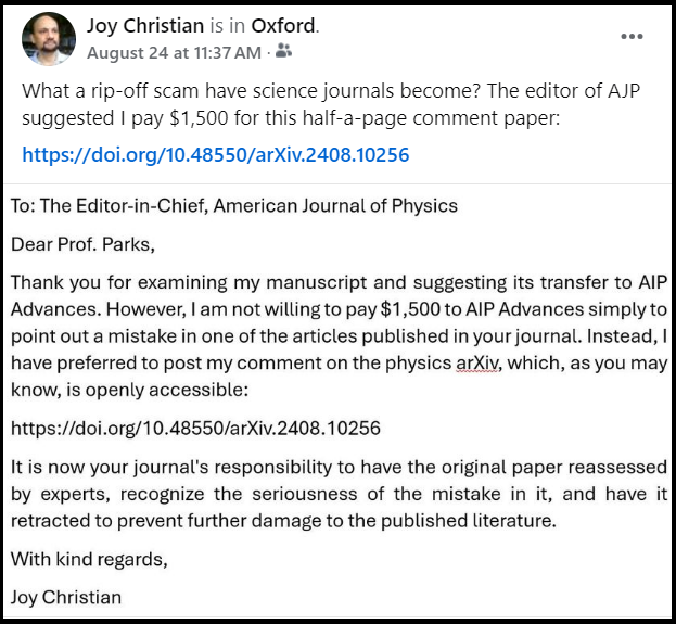
Why is this evidence so feared by the dark forces?
Bell’s theorem is entirely devoid of scientific merit.
It is merely a politically and sociologically sustained belief system.
In 1964 John S. Bell claimed to have proved a “theorem” that “no local and realistic physical theory (in the sense espoused by Einstein) can reproduce all of the statistical predictions of quantum mechanics.” However, in a series of papers written between 2007 and 2024 I have constructed just such a local and realistic theory for physics. As a result, today Bell’s theorem no longer has a scientific significance for physics it was once thought to have:

In a nutshell, my disproof of Bell’s theorem goes as follows: In 2007 I noticed that there is a serious error in the very first equation of Bell’s famous paper [Physics 1, 195 (1964)]. Bell simply made an elementary but fatal mistake, and this mistake lies in the formulation of the very first equation of his famous paper. The correct form of his proposed functions to reproduce the quantum correlations local-realistically must be

instead of

for them to provide a complete local description of the physical reality demanded by Einstein. The latter form, with 


Here the complete state 


It is very important to note that the image points of both forms (1) and (2) of the above functions, namely the measurement results 

.
with
![\displaystyle {\cal E}({\bf a})\,=\,\lim_{\,n\,\gg\,1} \left[\frac{1}{n}\sum_{k\,=\,1}^{n}\,{\cal A}({\bf a},\,{\lambda}^k)\right] \,=\,0\,. \ \ \ \ \ \ \ (4)](https://s0.wp.com/latex.php?latex=%5Cdisplaystyle+%7B%5Ccal+E%7D%28%7B%5Cbf+a%7D%29%5C%2C%3D%5C%2C%5Clim_%7B%5C%2Cn%5C%2C%5Cgg%5C%2C1%7D+%5Cleft%5B%5Cfrac%7B1%7D%7Bn%7D%5Csum_%7Bk%5C%2C%3D%5C%2C1%7D%5E%7Bn%7D%5C%2C%7B%5Ccal+A%7D%28%7B%5Cbf+a%7D%2C%5C%2C%7B%5Clambda%7D%5Ek%29%5Cright%5D+%5C%2C%3D%5C%2C0%5C%2C.+%5C+%5C+%5C+%5C+%5C+%5C+%5C+%284%29&bg=ffffff&fg=000&s=-1&c=20201002)
They are exactly what Bell assumed them to be in his first equation. Only the codomain of the two forms of the functions differ from each other. Failing to take the physically and mathematically correct codomain into account, Bell’s argument is thus indeed a non-starter. That is to say, his argument simply does not go through without the assumption of totally disconnected set 


![\displaystyle {\cal E}({\bf a},\,{\bf b})\,=\,\lim_{\,n\,\gg\,1} \left[\frac{1}{n}\sum_{k\,=\,1}^{n}\,{\cal A}({\bf a},\,{\lambda}^k)\;{\cal B}({\bf b},\,{\lambda}^k)\right] \,=\,-\,{\bf a}\cdot{\bf b}\,, \ \ \ \ \ \ \ (5)](https://s0.wp.com/latex.php?latex=%5Cdisplaystyle+%7B%5Ccal+E%7D%28%7B%5Cbf+a%7D%2C%5C%2C%7B%5Cbf+b%7D%29%5C%2C%3D%5C%2C%5Clim_%7B%5C%2Cn%5C%2C%5Cgg%5C%2C1%7D+%5Cleft%5B%5Cfrac%7B1%7D%7Bn%7D%5Csum_%7Bk%5C%2C%3D%5C%2C1%7D%5E%7Bn%7D%5C%2C%7B%5Ccal+A%7D%28%7B%5Cbf+a%7D%2C%5C%2C%7B%5Clambda%7D%5Ek%29%5C%3B%7B%5Ccal+B%7D%28%7B%5Cbf+b%7D%2C%5C%2C%7B%5Clambda%7D%5Ek%29%5Cright%5D+%5C%2C%3D%5C%2C-%5C%2C%7B%5Cbf+a%7D%5Ccdot%7B%5Cbf+b%7D%5C%2C%2C+%5C+%5C+%5C+%5C+%5C+%5C+%5C+%285%29&bg=ffffff&fg=000&s=-1&c=20201002)
is relatively easy to reproduce in a strictly local and realistic manner. In fact, once the topology of the codomain of the measurement functions 


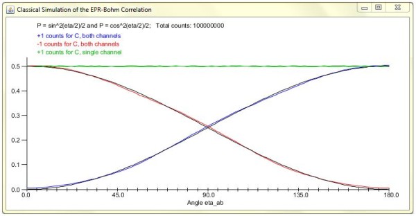
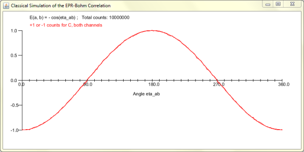
You can verify these facts in an explicit computer simulation of the model, as discussed in this paper. At least five explicit, event-by-event, numerical simulations of my local model for the EPR-Bohm correlation have been independently produced by five different authors, with codes written in Java, Python, Mathematica, Excel VB, and “R“. The above 2D-surface version of the simulation of my local model can be found here. I discuss two of these simulations in the appendix of this paper. A compact translation of one of these simulations (from Python to Mathematica) can be found here. Each simulation has given different statistical, geometrical, and topological insights into how my local-realistic framework works, and indeed how Nature herself works.
The most accurate simulation of my local model for the EPR-Bohm correlation can be found here.
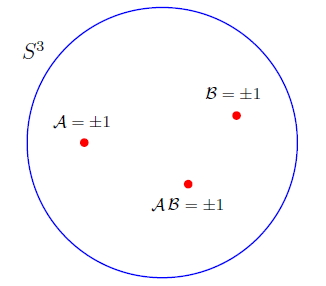
From the above discussion Bell’s mistake is now very clear. Instead of investigating correlation among the points of a parallelized 3-sphere, Bell naïvely investigated correlation among the points of a real line to prove his celebrated theorem. But even an elementary topological consideration is sufficient to recognize the fact that correlation among the points of a real line cannot possibly be the same as those among the points of any topologically nontrivial space such as a parallelized 3-sphere.
But what about the famous Bell-CHSH inequality on which Bell’s supposedly iconic theorem is based? It turns out that it too can be violated local-realistically. In doing so, however, we gain a tremendous insight into the very origins of quantum correlations. This is discussed in greater detail on the next page, but first let us recall that for the set of four measurement directions, a, a

provided we assume the corresponding measurement functions to be of the incorrect form (2) assumed by Bell. Thus it is in this step—the crucial step in the derivation of Bell-CHSH inequality and the proof of Bell’s theorem—that the assumption of incorrect codomain gets smuggled-in. The four pairs of measurement results occurring in the above expression clearly cannot all occur at the same time. If, however, we conform to the usual assumption of counterfactual definiteness and pretend that they do all occur at the same time at least counterfactually, then we must specify the correct codomain for the functions 


![\displaystyle \leqslant\sqrt{\,\lim_{\,n\,\gg\,1}\left[\,\frac{1}{n}\sum_{k\,=\,1}^{n}\, \big\{\,4\,+\,4\,{\cal T}_{\,{\bf a\,a'}}({\lambda}^k)\,{\cal T}_{\,{\bf b'\,b}}({\lambda}^k)\,\big\}\,\right]} \ \ \ \ \ \ \](https://s0.wp.com/latex.php?latex=%5Cdisplaystyle+%5Cleqslant%5Csqrt%7B%5C%2C%5Clim_%7B%5C%2Cn%5C%2C%5Cgg%5C%2C1%7D%5Cleft%5B%5C%2C%5Cfrac%7B1%7D%7Bn%7D%5Csum_%7Bk%5C%2C%3D%5C%2C1%7D%5E%7Bn%7D%5C%2C+%5Cbig%5C%7B%5C%2C4%5C%2C%2B%5C%2C4%5C%2C%7B%5Ccal+T%7D_%7B%5C%2C%7B%5Cbf+a%5C%2Ca%27%7D%7D%28%7B%5Clambda%7D%5Ek%29%5C%2C%7B%5Ccal+T%7D_%7B%5C%2C%7B%5Cbf+b%27%5C%2Cb%7D%7D%28%7B%5Clambda%7D%5Ek%29%5C%2C%5Cbig%5C%7D%5C%2C%5Cright%5D%7D+%5C+%5C+%5C+%5C+%5C+%5C+%5C+&bg=ffffff&fg=000000&s=0&c=20201002)


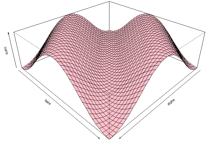
This upper bound has been derived in detail in the last appendix of this paper. This derivation has also been numerically verified in a GAviewer by Fred Diether and myself. It is of course exactly what is predicted by quantum mechanics. Thus, with the topologically correct choice (1) for the measurement functions, not only the strong correlations (5) but also the upper bound (7) on the correlations turns out be exactly what is predicted by quantum mechanics.
More importantly, the above derivation reveals a crucial role played by the non-vanishing torsion in our physical space on the strength of the observed correlations. If the physical space in which the measurement events 

Needless to say, the above discussion is merely a sketch of my disproof. In particular, I have glossed over the important issue of how errors propagate within a parallelized 3-sphere (a detailed statistical analysis of which can be found in this paper). Moreover, in my book I have shown that, not only the simple EPR-Bohm-type correlations, but ALL quantum correlations can be reproduced purely local-realistically in an analogous manner. For more general cases, however, the codomain of the measurement functions such as 

The argument I have presented above is experimentally testable. I have proposed a macroscopic experiment for this purpose. Further discussion about this experiment can be found on this page.
PS: A theoretical computer scientist, Paul Snively, has crystalized the essence of my argument in a logical sequence that I find quite interesting. According to Snively the logic behind my refutation of Bell’s theorem is:
algebra with operations lacking the closure property 
A brief discussion of what he means by this sequence can be found on this page of his blog.
He summarizes the main point thus: “Dr. Bell used scalar algebra. Scalar algebra isn’t closed over 3D rotation. Algebras that aren’t closed have singularities. Non-closed algebras having singularities are isomorphic to partial functions. Partial functions yield logical inconsistency via the Curry-Howard Isomorphism. So you cannot use a non-closed algebra in a proof, which Dr. Bell unfortunately did. … This is a sufficient disproof of Bell’s theorem.”
Let me add to Paul’s observation that, not only Bell’s original 1964 proof, but *ALL* of the proofs of *ALL* of the Bell-type theorems, including the proofs of their variants and generalizations such as Hardy’s theorem or GHZ theorem, use only scalar algebra. Therefore all such no-go “proofs” are logically inconsistent (i.e., they are nonsense).
———-
Bell has been credited for discovering the mistake in von Neumann’s “no hidden variables” theorem even though both Einstein and Grete Hermann had discovered von Neumann’s mistake some 30 years before Bell did.
Now Bell does have a nice and succinct explanation of von Neumann’s mistake in section 3 of the first chapter of his book. At the end of his section 3 Bell says something that is quite ironic in my view.
Bell writes: “Thus the formal proof of von Neumann does not justify his informal conclusion. … It was not the objective measurable predictions of quantum mechanics which ruled out hidden variables. It was the arbitrary assumption of a particular (and impossible) relation between the results of incompatible measurements either of which might be made on a given occasion but only one of which can in fact be made.”
How ironic! That is precisely the mistake Bell himself has made in his own famous theorem, as I have explained in section 4 of my Royal Society paper and in these preprints.
————————————————————————————————————
![]()


Hi Joy,
I was just looking at this video on the Scientific American website about quantum entanglement presented on a blog by George Musser. I have to say that after understanding your model, I could immediately see where the argument for quantum entanglement breaks down in the video. I am wondering if anyone else reading this blog can point out those spots in the video?
I remember on the FQXi blogs that George Musser noted to you that he would like to have a better discussion with you about your model. I think it is only fair that a counter opinion about quantum entanglement should be offered to SciAM readers and you should take George up on his offer.
Best,
Fred
Hi Fred,
I watched the video. I must admit I am deeply disappointed and disturbed by how misleadingly the idea of entanglement is presented in the video. With all due respect to George Musser (who I think is a talented young journalist), what he is doing is no different from “spreading the good word” of entanglement. The video is misleading from the start. The two men set out to witness entanglement firsthand in a physics lab. But you can no more witness entanglement of a photon than you can witness phlogiston in a combustible body. All one can ever see in a lab are correlations between the supposedly entangled photons. No one has ever seen, or could ever see, entanglement directly. If we could, then all controversies over the interpretation of quantum mechanics would end instantly.
To be sure, we can prepare various states of the photons as shown in the video—say, a state in which the correlations exhibited by the photons is no better than that produced by coin tosses, or a state in which the correlations exhibited by the photons which can be explained by the concept of entanglement. But the latter is not the only explanation possible for the observed correlations, as we know from the results of this paper. I show in this paper how the observed correlations can be explained without the notion of phlogiston… I mean entanglement. They can be explained simply as classical, deterministic correlations among the points of a parallelized 3-sphere. So it is very disappointing indeed that Scientific American would continue to “spread the good word” of entanglement without even mentioning the much less mystical alternative. The day will come, however, when the idea of entanglement would be no more in vogue than the idea of phlogiston.
Best,
Joy
Hi Joy,
I appreciate your remarks and do hope to continue our discussions at some point. But I think you will admit that your views on entanglement are a minority opinion. Of course that doesn’t make them wrong! The history of science shows that minority opinions are often vindicated; all great truths are initially resisted. Nonetheless, Scientific American *has* to give higher weight to prevailing views — otherwise, the editors would be placing their own judgment above that of the majority of scientists, which is sometimes justified, but only in exceptional cases. To put it differently, once you convince your fellow physicists and philosophers of physics of your arguments, then you will have convinced us, too.
George
Hi George,
Thanks for dropping by and responding to my comments. I do agree that my views on entanglement are a minority opinion at the moment, and I do appreciate why Scientific American has to give higher weight to the prevailing views. But it seems to me that your video linked above gives a wrong impression of entanglement even from the prevailing point of view. It is understood by most experts (say, by Lucien Hardy, for example) that all we can see in the lab are correlations, not entanglement itself. The latter concept provides a good explanation for the observed correlations, but that is a different matter.
But again, I appreciate that you have a short time at your disposal in which you have to explain the essence of the idea to lay viewers, without getting into technicalities.
As for my own views on entanglement, I do hope that someday my arguments are better understood by my fellow physicists and philosophers of physics. In any event—leaving your journalist hat aside—please feel free to continue the discussion we started during the last FQXi conference.
Best,
Joy
I hope our world lines will intersect soon, so that we can continue our chat. Please let me know if you have plans to visit NYC.
George
Hi Joy,
I’d like to expand on the phlogiston example you used. Shorly before Lavoisier showed that combustion is caused by rapid oxidation, there were theoretically two kinds of phlogiston, deduced from the evidence of combustion — “positive” phlogiston in the form of rust, which apparently added matter to a substance such as iron, and “negative” phlogiston which apparently subtracted matter from a substance such as wood, which was reduced to ashes.
These conclusions are of course contradictory. The contradiction is of the same form [as certain mistaken claims about] your framework. Just as “phlogiston theorists” were mistaken about the true nature of combustion, so are these [claims] about the constructive nature of a continuous measurement process that obviates the identification of discrete outcomes with physically real, nonlocal results.
Best,
Tom
Hi Tom,
Thank you for your comments. I did not know that there were two kinds of phlogiston.
I am terribly sorry, however, because I had to edit out parts of your message. Names of certain individuals whom I cannot respect are not allowed on this blog. I hope you will understand. I have tried to preserve the integrity of your message as much as possible.
As for the mistaken claims of those individuals you mention, it is important to note that equations (1.22) to (1.26) on page 10 of my book, as well as similar set of equations in this paper, have been explicitly verified (in great detail) by Lucien Hardy, Manfried Faber, and several other high profile and exceptionally competent physicists and mathematicians around the world. In fact, any competent reader with only basic skills in mathematics should be able to reproduce equations (1.22) to (1.26) of my book rather effortlessly.
It is also worth noting that all of the so-called arguments against my disproof to date are based on an elementary logical fallacy—the Straw-man Fallacy. What they do is replace my argument (or model), say X, with a grossly distorted misrepresentation of it, say Y, and then pretend—by refuting their own distortion Y (by resorting to deliberate dishonesty or out of sheer incompetence)—that they have undermined my actual argument (or model) X. Such a dishonest strategy defies reason at its very core (for more details, see this paper).
Unlike Bell himself, some of the followers of Bell are naïve, uninformed, and dishonest.
Best,
Joy
Hi Joy,
The presence of positive and negative phlogiston is implied in the link you gave. The author just failed to point out the contradiction between two *physical* results from a theory that can accommodate only a singular physical outcome. If phlogiston is assumed to be physically real, it must be causal, and if causal, attributable to only one result. It doesn’t do to say that in the one case phlogiston causes rust and in the other case, causes ashes. If rust and ashes have a common cause, it can’t be phlogiston.
By the same token, non-vanishing topological torsion analogous to the rapid oxidation that causes both rust and ashes, informs us that continuous functions imply classical orientation entanglement — (and not the entanglement of real physical quantities whether we call the phenomena phlogiston or quantum entanglement) — that guarantees a unitary cause.
In other words, if one assumes phlogiston, an experimental outcome of + 1 (rust) or – 1 (ashes) explains nothing. Both (contradictory) outcomes can’t result from the same physical cause. Your topological model, OTOH, has the same attributes as chemical oxidation in principle: a continuous process drives the measurement result from a deeper underlying physical cause of nondegenerate torsion.
Einstein faced the same problem in explaining how spacetime is physically real (” … independent in its properties, having a physical effect but not influenced by physical conditions…”) because one does not think of continuous phenomena as physically real. One intuitively wants to ascribe “reality” to the measurement apparatus rather than the measurement process.
Your critics are not subtle thinkers. They allow that 2 and 3 dimensional simulations are adequate for n-dimension phenomena. Thus, they reject *any* topological model out of hand; global results, as topology implies, have to be nonlocal by definition. I think that until one can grasp the analytical nature of your framework, it’s an uphill battle. Einstein had the advantage of large scale validation for continuous spacetime. Small scale classical experiments are tougher, less forgiving. Just as one has to accept a 4-dimension physical spacetime continuum for general relativity to make sense, one has to accept a parallelized physical 7-sphere for your framework to make sense. And just as Minkowski space-time requires a great deal of mathematical background to grasp, your framework requires that much more.
Best,
Tom
Hi Tom,
You make some very good points. Sadly, as you put it, my “critics are not subtle thinkers”, to say the least. Moreover, dogmas, even within science, are not easy to overcome, as we have witnessed over the past few years. But thank you for your thoughtful remarks, especially concerning the phlogiston analogy.
Best,
Joy
Hello
I have on my website 2 formulae that work with good performance at the degree resolution level. There is an online and checkable javascript implementation for the ones that haven’t a tool to emulate probability functions and to compute correlations.
any advice is welcome 🙂
Hello Igael,
What you have is a nice demonstration of well known facts. It is well known (since 1970’s) that by reducing the efficiency of detection, to, say, 86%, one can reproduce the cosine correlation. Such a demonstration does not contradict Bell’s argument, and it does not have fundamental significance for physics.
Best,
Joy
Hi
Please note that I’m working on new variants with 89% pairs ( then 94% of arm efficiency ) and probably more. I use 80 servers , raising to ‘powers’ above 3.000.000.000 without Markov takes a lot of resources
But, you are true , even if I haden’t yet seen theses formulae on sites or books.
It is not so clear when you read QM curses or books on EPR to understand that the debate is not closed. How to start developping applications in such conditions ?
Please, let me know where I could find the formulae known since 70 ? I found only the Maudlin scheme B ( it seems to my algo 9 without Markov and has a limit around 66.6 % pairs and not 63.6 as I read in some articles ) ?
This is an amazing topic !
Thank you.
Igael
Igael,
I had this paper in mind: Hidden-Variable Example Based upon Data Rejection, by P. Pearle, Physical Review D 2, 1418–25 (1970).
Best,
Joy
Hi Joy
Many thanks.
Hi Joy.
BLOG: (revise or cut as you wish)
Eureca!
I found your decorative blog.
Checking ‘Internet’ it appears that you have been through some nasty ‘entanglements’ and have passed it in ‘local reality’, free and well, – with honour.
Good luck for your further work!
engaged Emeritus.no
PRIVATE:
If you check your e-mail box for 03.03.2014, Re: Bell’s theorem, with two enclosed items, you will find the background for my contact.
I would appreciate v.m. a reply and a comment to my paper. ( I can repeat the e-mail if you have lost it).
w.f.g. Olav
Linear Polarization http://vixra.org/pdf/1303.0174v5.pdf
Einstein was right when he did not agree with the EPR experiment conclusions and had said, “spooky action at a distance” cannot occur and that, “God does not play dice”.
Electron Spin
http://vixra.org/pdf/1306.0141v3.pdf
Dr. Christian,
I would imagine Tom Ray might keep in touch with you, so you might know that the current FQXi essay contest has an entry by Edwin Eugene Klingman in which he challenges constraints inherent in Bell’s formulation, which produce the same distribution curve against the Bell straight-line eigenvector that your topological challenge results in. Not that I blame either you or Tom for not continuing to subject yourselves to the abuse of the blogosphere, I think it wise. I recall warning R. Gill that his posturing in Vienna made him a perfect fall guy for professional spooks. I had wondered if he ever made it back from his ‘sabatical’ to the Baltic, hope you actually collected the 10K Euros. Kudos, jrc
Dr Christian:
You are a diseased little turd swirling around the toilet drain en route to an obscurity even deeper than the one currently defining you.
Sincerely
Thank you, Mr. Rosenblum.
If your prophesy is right, then there is no reason for you to be concerned. 🙂
Dr. Christian,
As I understand (interpret) your theoretic conjectures, the problem arises from the interpretation of what a particle represents: QT versus your description – point vs 3D object (sphere), wave of probability with instantaneous communication between points in ST versus local ST with light speed limitation. I have always wondered how points in QT (Copenhagen Interpretation) can possess complex properties and give rise to complex interactions? QT begs for existence of hidden variables.
Do waves of probability also govern virtual particles? And how could we unite the Copenhagen interpretation with your view?
The answer could very well lay in an existence of a real De Broglie wave made of two sets of virtual photons (intersecting at opposite directions and at the speed of light) which express their circular polarization pattern only at a “point” at which the particle (the Higgs expression?) is located. Those photons would cancel to randomness in all other positions along their path of propagation, and shifting their frequency would lead to particle speed change. In this view matter would be a stable interference pattern. Particles would form as rain drops form in clouds and would exist intermittently pulsating to the beat frequency of the waves that build them.
So, does this expression fit yours?
Also you could have a look at the work of Dr. Yves Couder: https://www.youtube.com/watch?v=W9yWv5dqSKk
Cheers!
We have finally launched the long-awaited website for the Einstein Centre for Local-Realistic Physics: http://einstein-physics.org/.
I have posted a simplified version of my proposed macroscopic experiment to test Bell’s theorem here: http://libertesphilosophica.info/blog/wp-content/uploads/2016/05/PropExp1.pdf.
Joy, I am reminded of Robert Jay Lifton’s book on ideological totalism, especially chapter 22 where it talks about the demand for purity. A hilarious video mocks cult behavior with a scene where the indoctrinated mob repeatedly chants “stamp out doubt.” Frankly, these people couldn’t connect Back to the Future to The Walk (lol) but I digress… The problem I have with criticism of your work is that it’s religious in nature and the people conducting the criticism are frankly not qualified enough to be passing judgment. For such a prominent issue, we need prominent referees, especially given the novel math employed. Journals are a joke these days, so I don’t accept their vetting on such a novel argument. The reproducibility crises reveals they are in a massive credibility meltdown and can’t be trusted in an age of hyperspecialism and information overload. What surprises me is that the actual physics community has been afraid to directly engage you. Getting a self-righteous statistician in the Netherlands to do it for them is quite cowardly and comical, even if he’s right. Vicious blog trolls like Luboš Motl (long disgraced from the physics community) just copy-and-paste criticism and confess ignorance of geometric algebra, as did Gill. This is the same community that endorses the multiverse, SUSY, unprovable black hole theories, quantum computers and non-empirical string theory and E8 speculations. The entire profession is becoming an inside make-work joke. In my opinion, it’s a funding bubble that never got popped since WWII but I digress again… QM just gives expectations of observables and probability is merely an interpretation (the Born rule is “metaphysical fluff”). Amplitudes interfere and not probabilities (the wave function can be positive, negative, complex, spinor, or vector ), so I think quantum computers do not even follow directly from QM but those like Aaronson refuse to acknowledge any doubt. I admit that there is no reason to conclude that quanta must necessarily be reducible to traditional math at all because the map is not the territory but I digress again… A very clear and basic explanation of the reason why Bell’s theorem doesn’t imply non-locality has just been published and two points can be made immediately from the paper: measurements are not predetermined or (second hidden conclusion) traditional math can’t model quanta and QM is incomplete. In other words, one can reject a naive version of “realism” to get rid non-locality. What is really nice about this paper is that it can be read by just about anyone. Your serious error is the error of arrogant academia in general, which is a lack of self-contained explanations. Take someone from a high school linear algebra, calculus and physics background to the endpoint of your argument without skipping steps. Clarity is key. You spend more time answer trolls than explaining things to the rest of us. It would be time better spent!
Many thanks for your comments. I agree with much of what you have written. It is indeed true that I have spent too much time answering ignorant and self-righteous trolls like Gill.
There is some good news, however. One of my latest and comprehensive papers has just been published by the Royal Society of London in their journal Open Science: http://rsos.royalsocietypublishing.org/content/5/5/180526
So, finally, some well-qualified people had a chance to look at my argument closely and have approved the publication of my latest paper, in a prominent journal. 🙂
Seeing you wrestle with Gill reminded me of the fight scene from John Carpenter’s They Live (ROFL!). While your argument against Bell is about topological incompleteness, Marian Kupczynski has a different approach to give a local realist account: “The oversimplification made by Bell was the assumption that Λxy= Λ =Λ1 x Λ2 what is equivalent to assuming that the correlations in different incompatible experiments may be deduced from a joint probability distribution on some unique probability space Λ.” Rather simple. I was always skeptical about a hyper-generality of Bell’s theorem because problems of reality are so open-ended. People should be jumping up and down with “joy” to see their way beyond Bell.
I agree with the argument that “The oversimplification made by Bell was the assumption that Λ = Λ1 x Λ2, which is equivalent to assuming that the correlations in different incompatible experiments may be deduced from a joint probability distribution on some unique probability space Λ.” The philosopher Arthur Fine pointed this out many decades ago. And yet the mainstream Bell community has been ignoring this obvious weakness in Bell’s argument. They do not seem to understand the simple logic that if you put garbage in a theorem, then all you can expect to get out of it is also garbage.
Hello Dr. Christian, have you ever heard of Eric Reiter? He’s been doing quantum physics experiments for the last 20 years. Published results, has videos of his work and collection of writings in freely available book. All here
https://www.thresholdmodel.com/
He claims to have found the error in all quantum experiments which when accounted for experimentally, removes the quantum effects and their associated ghosts. No superposition, no spooky action at a distance, no Bell, etc.
Basically, Planck should have stuck with his second threshold model and extended it instead of going with the quantum one. Take a look and see if Eric is right.
Hello Mark,
Thank you for your comments. Yes, I have known Eric Reiter via social media, and we also had some correspondence via email.
I cannot comment on Eric’s experimental work because I am not an experimentalist. However, I would be very surprised if Eric has found a genuine error in quantum experiments. The predictions of quantum mechanics have been verified, not only for one or two physical phenomena but for a huge variety of physical phenomena, from radiation theory to solid-state physics, to elementary particle physics, for over a hundred years, in hundreds of thousands of experiments. It is of course not impossible that Eric may have found an anomaly in some of these experiments, but, as I once told Eric, he must have these anomalies verified independently by some of the respected experimentalists. Anomalies are often found in physics. But most of them disappear after careful examinations. In any case, no anomalous experimental claim would be accepted by the physics community unless it had been verified independently.
Incidentally, I do not question quantum mechanical predictions in my work, just as Einstein never doubted the validity of quantum mechanics. With Einstein, what I reject is the Copenhagen and related interpretations of quantum mechanics. From what little I know of Eric’s work I am not persuaded that there is anything wrong with the predictions of quantum mechanics. What is wrong is some of the bogus interpretations of quantum phenomena, inspired by Bell’s theorem. In my view, Bell’s theorem is a fundamentally flawed argument.
Thank you Dr. Christian, that helps me a lot. I am not a physicist but is it possible for you to explain in more laymen’s or at least undergraduate student terms what is the problem with Bell’s theorem, which interpretations of quantum theory it applies to and which not and the interpretation you prefer. Thanks again.
Bell’s theorem purports to prove that Einstein’s statistical interpretation of quantum mechanics, which resolves all its seemingly unpalatable features, is not viable because such an interpretation would necessarily involve non-locality. But Bell’s theorem is a circular (and thus a fundamentally flawed) argument. It assumes in its premisses what it sets out to prove. In technical terms, it assumes that we can add expectation values of random variables even when these variables cannot be measured simultaneously. Thus, the mistake in Bell’s theorem is quite elementary. And since Bell’s theorem is fundamentally flawed, Einstein’s statistical interpretation of quantum mechanics is perfectly viable, without any undesirable features.
The videos are published now with your suggested corrections Joy! We decided to split the video in to 2 parts to be more digestible. The channel is the same as before. It seems it is already bringing attention to your blog 🙂 can’t wait to finish the 3-sphere part, but it’s going to take a while.
Thank you, Sandra. And congratulations on completing the first two parts. I look forward to watching them.
Hi Joy. While doing the research for the final part in the series I looked up older papers like your replies to critics. In “Refutation of Some Arguments Against my Disproof of Bell’s Theorem”, you reply to Moldovenau. Here, you make a statement:
.
“Usually one expects the numbers A and B to change when the directions of measurements a and b are changed. This informal expectation, however, is profoundly misguided. No such local contextual change is ever observed in the actual experiments, or even predicted by quantum mechanics.”
.
You are saying that your model is non-contextual. Aren’t non-contextual models ruled out by the Kochen-Specher-Theorem?
.
But then, in “Dr. Bertlmann’s Socks in the Quaternionic World of Ambidextral Reality”, you say: “two different vectors a and a′ chosen by Alice may correspond to the same measurable quantity A , measured along different contexts, without reference to what is measured on particle 2; and likewise for Bob. Therefore the hypothesized hidden variable theory is locally (but not remotely) contextual.”
.
.
These two statements appear to contradict each other, but are dealing with the same model. Could you clarify the nature of these statements?
Hi Sandra,
Good question. There is a peculiar property of the earlier Geometric Algebra model that makes it manifestly non-contextual. You can see that from the equation (36) or (37) in Section V of my reply to Moldoveanu. If you change the vector a to a’ in equation (36), then the result, +1 or -1, does not change. This is because, in that early model, I had not yet been using the limit process that is used in equation (39) of the “Dr. Bertlmann’s Socks” paper. So, the limit process brings the early model closer to the traditional Bell model. It then becomes subject to the Kochen-Specker theorem that rules out non-contextual theories. Since the later model with the limit process is closer to physics in the experiments, it is best to stick to it for now, leaving the issue of non-contextuality of the earlier model for future investigations. Ideally, I would like the 3-sphere model to be strictly non-contextual as Einstein wanted. But I have not been able to square that circle yet.
Hi joy, a recent comment I received states the following:
“The traditional CHSH quantity is (+1)AB + (+1)AB’ + (+1)A’B + (-1) A’B’. Since you insist on using non-commuting objects, you also implicitly have (+1) in between each pair of outcomes, and even (+1) after each pair of outcomes. There’s also implicit coefficients of 0 in front of terms linear in each of these outcomes that weren’t needed for the choice of zero-centered measurement outcomes. But take a step back from there, even, and address the simpler task of where you were trying to assign one of only two possible values to A. Given whatever two distinct quaternion values you chose, you can find an expression c A d + e that takes on 1 or -1 values. Then you plug in those expressions you found into the standard CHSH quantity, and you find the best constraining CHSH-type quantity for your quaternion-valued case.”
.
How would you respond to this? I’m not sure I even understand the argument.
The problem with social media discussion is that the quality of comments is not always guaranteed. The commentator has not understood your argument. We are not insisting on inserting non-commuting objects in the CHSH quantity. We are saying that the commuting numbers, A = +/-1, B = +/-1, etc., that traditionally appear in the CHSH quantity are *eigenvalues* of *non-commuting* quantum mechanical operators. As such, they cannot be added (or summed up) as is traditionally done in the CHSH quantity to give the correct bounds on their CHSH sum. In other words, the traditional CHSH quantity is entirely irrelevant for the Bell-test experiments in which eigenvalues of *non-commuting* operators are inevitably observed, because of the experimental impossibility of observing the eigenvalues, AB, AB’, A’B, and A’B’, simultaneously.
I believe the commenter said this because I showed how, giving the functions like A(a,lambda) unit quaternion values, we can reproduce the quantum mechanical result. A physical reason i gave for this is that different directions of measurement physically correspond to different orientations in space (so that those +1 and -1, although being the same numbers, must under the hood encode this difference), and to describe orientations we cannot use scalars.
.
The commenter insisted that “Once you expand the scope of what values the measurements can have, you need to also expand the scope of what the coefficients are so that you can find the new most constraining inequality.” and “No, we should use the one that gives the strongest constraint on a local theory. Even if you want to insist on using a different definition and using unit quaternions, then you have to find the best bound over all CHSH-type quantities, which means inserting quaternion coefficients in various places. Then you’ll arrive at the same conclusion that everyone else already reached more easily with +1 and -1 values.”
.
I’m asking you Joy because since i’ve never heard of this “coefficient” argument I might be misrepresenting your work.
Let us first sort out what you are saying. Show me, or point me to, where you have made your argument. I know you are trying to explain things by simplifying my technical arguments, but that would very likely lead to misrepresentation. So, let me first understand what you are saying before worrying about what the commentator is saying. To be frank, that comment by someone you quoted earlier seems gibberish to me.
Thank you Joy for being so available, and sorry if you find i’ve misrepresented you. I’ve been trying to spread the word on social media, with mixed results.
This is where the thread starts: https://www.reddit.com/r/quantum/comments/1farfd9/comment/llx4kjy/?utm_source=share&utm_medium=web3x&utm_name=web3xcss&utm_term=1&utm_content=share_button
Ok. This is a long thread, so it will take me some time to read it. But some of the things you say there are correct and some are not. For example, Bell did not make a mistake in assuming that the measurement results are scalar quantities. Of course they are scalar quantities. They are just +1 and -1 numbers. What is wrong with his argument is that these scalar quantities are actually eigenvalues of non-commuting operators, and therefore they cannot be added linearly, just as von Neumann should not have added expectation values linearly in his theorem. So, at some places, you are explaining this correctly. The other guy gets confused when you bring up orientations and quaternions. So the best strategy is to keep the discussion about Bell inequality separate from that of the correlations derived within a quaternionic S^3, especially on social media. If I have more comments after reading the thread I will add them here. But for now, just keep these two things — Bell inequality and orientation of S^3 — separate, and you will be fine.
I think it’s appropriate to ask you if this is correct then, since I was planning to add a section like this in part 3 of the videos. The point i was trying to make with that “these can’t be scalars” is that since they don’t obey linear additivity as eigenvalues (which indeed are always scalars in quantum theory), the respective +1 and -1 obtained from functions like A(a,lambda) must reflect this algebraic property. This means such a function cannot return strictly scalar values, but should be instead thought of a quaternion based function (or alternatively bivector valued). Similar to your limiting function on bivectors, we can take any quaternion like q(0, s) to reduce it to a limiting scalar value, but once we multiply two such “scalars” we end up with a unit quaternions which is not strictly a scalar.
.
q(0,s)q(0,t) = s*t + (s x t)
.
This should not be a problem at all, since quantum mechanics does not tell us what the value of the product AB is for a single measurement. It merely tells us, through a tensor product, that the average of this product will be the dot product of the two vectors.
.
Depending on the orientation of the 3-sphere, we can also have the inverse product, which simply returns the same value with a negative sign before the cross product.
.
q(0,t)q(0,s) = s*t – (s x t)
.
Averaging over them for N particle pairs we get the quantum mechanical prediction of s*t.
In the eigenvalue formalism, the product of operators AB is still +1 or -1 only for the fact that experiments don’t allow us to tell the absolute orientation of the measurement, meaning in our experiments A and B commute. In general the product of two spin operators on the same particle would yield a non-scalar value.
.
The upper bound for the quaternion expression would be, for the four angles,
.
A*B + (AxB) + A*B’ + (AxB’) + A’*B + (A’xB) – A’*B’ – (A’xB’).
.
Which, for angles AB, A’B, AB’ = 45° and A’B’ = 135° like in the maximally entangled state, becomes
.
√2+ab(1) + √2 +ab'(1) + √2 +ab'(-1) – √2 – a’b'(1)
.
Where the small letters simply represent the orthogonal vector from the cross product.
It’s easy to see that ab and a’b’ are colinear vectors, so they cancel out, leaving us with 2√2.
.
I’m using quaternions instead of bivectors simply because it’s easier to connect them to the concepts of division algebras, which in turn are connected to the n-spheres. I still plan on mentioning the use of geometric algebra at the end, but only as a simplification of the formalism and for giving geometric intuition.
Unfortunately I can’t edit the comment! In the last expression the number between parenthesis like ab(1) should be √2, not 1. The end result is the same.
Sorry for spamming, i really wish i could just correct the comment itself. I though i should just rewrite the expression since I got quite a few mistakes in it:
.
√2+ab(1) + √2 +ab’(1) + √2 +ab’(-1) – √2 – a’b’(1)
.
Should be
.
√2+ab(√2) + √2 +ab’(√2) + √2 +a’b(√2) – √2 – a’b’(√2)
.
ab and a’b’ are collinear and with the same orientation, so they cancel out. ab’ and a’b are also collinear, but with opposite orientation, so they cancel out as well.
Gosh! Of course its not
.
√2+ab(√2) + √2 +ab’(√2) + √2 +a’b(√2) – √2 – a’b’(√2)
.
but
.
1/√2+ab(1/√2) + 1/√2 +ab’(1/√2) + 1/√2 +a’b(1/√2) + 1/√2 – a’b’(1/√2)
.
I did not sleep well tonight!
Hi Sandra,
You say:
“The point I was trying to make with that “these can’t be scalars” is that since they don’t obey linear additivity as eigenvalues (which indeed are always scalars in quantum theory), the respective +1 and -1 obtained from functions like A(a, lambda) must reflect this algebraic property. This means such a function cannot return strictly scalar values, but should be instead thought of a quaternion-based function (or alternatively bivector valued).”
No. This is not strictly correct. The failure of linear additivity does not imply that the eigenvalue functions A(a, lambda) representing the measurement results themselves must be non-scalar. It means that the expectation functions for dispersion-free states of any hidden variable theory cannot be added linearly. It means that the sum of the expectation values of several operators cannot be equal to the expectation value of a sum of those operators. But each expectation value still just gives a scalar number: +1 or -1. See my paper for a detailed discussion: https://doi.org/10.48550/arXiv.2302.09519
Then you say:
“This should not be a problem at all, since quantum mechanics does not tell us what the value of the product AB is for a single measurement. It merely tells us, through a tensor product, that the average of this product will be the dot product of the two vectors.”
But in experiments, the product AB, which represents the joint measurements by Alice and Bob, is always equal to either +1 or -1, because A and B are observed to be +1 or -1.
The rest of your manipulation using quaternions will not go well with those who believe in Bell’s theorem. They will point out that Bell inequality is about experimental results and experimental results only: A = +1 or -1, and B = +1 or -1. If we use any non-scalar quantity then it is easy to reproduce the strong correlations and the bound 2\/2 on the CHSH quantity.
So, I am afraid, the simplified explanation you intend to make, which you and I fully understand, will not be understood or accepted by any diehard Bell believer.
Ok, Bell’s theorem is simply a non-sequitur for that reason, period.
.
But then we still need to model the correlations. For spin measurements we have directionality, and this can be intended as orientations in a 3-sphere. So it’s just in this context that we can use quaternions/GA?
.
I’ve recently come to know other types of entanglement experiments that don’t involve directionality at all, like time-bin experiments involving “time of flight” of photons, or quantum dots. I thought I had an intuition now for how GA represented orientation entanglement, but these experiment don’t seem to involve that at all.
Yes, Bell’s theorem is simply a non-sequitur, and Bell inequalities are therefore irrelevant.
In modeling correlations, it is worth remembering that not all correlations are as strong as those predicted by the singlet state. The 2\/2 strength of the correlations is the strongest possible strength of any correlations predicted by quantum states. This was proved by the late mathematician Boris Tsirel’son. Thus, the directionality and orientations of the 3-sphere are needed only for the correlations of strengths greater than the bounds of 2 on the CHSH quantity. For the rest, such as those involving the “time of flight” of photons or quantum dots, the ordinary R^3 model of the physical space would suffice. Moreover, for those correlations that are stronger than the bounds of 2 on the CHSH quantity, we have the general 7-sphere framework (published in my Royal Society papers). That framework, although more complicated than the 3-sphere model, accommodates a local-realistic understanding of all possible correlations predicted by any general quantum state.
It is also important to remember that the purpose of a hidden variable interpretation is not to replace quantum theory but to provide a local-realistic foundation to it, similar to how statistical mechanics provided a deeper foundation for thermodynamics without replacing it.
Quantum dots and time bin experiments violate the inequality still. The measurements are not direction measurements like in spin polarization EPR tests, rather they use interference through a Mach-Zender interferometer. It’s time-energy entanglement.
.
https://www.nature.com/articles/s41567-024-02543-8
.
But here’s the funny thing: I was worried by this since it appears we can’t model with S3 something that is not direction-dependent like interference. Then I looked up the supporting information.
.
https://static-content.springer.com/esm/art%3A10.1038%2Fs41567-024-02543-8/MediaObjects/41567_2024_2543_MOESM1_ESM.pdf
.
Turns out that to select the appropriate phase to measure through interference, they used… You guessed it… A polarizer.
Thank you for this information. I haven’t paid much attention to such experiments since I am usually put off when they mention “violations of Bell inequalities”, non-locality, etc. Such claims are utterly misguided in my view. Nothing “non-local” is going on in Nature.
Keep looking into such publications and find their hidden assumptions. Sometimes it takes a long time to figure out their missteps and mistakes. For example, I have worked on the GHZ theorem before, reproducing (in 2009) all of the predictions of the 3- and 4-particle GHZ states within the 7-sphere framework. But only recently I discovered the mistake in the GHZ argument itself, which I have now published in the one-page comment paper I linked above.
Hi Joy!
Slightly different question from usual: how does providing a local realistic hvm affect the field of quantum computing? I’m far from an expert on that, but I have seen your past posts on it and some words by Mikail Dyakonov. While I understand the practical issue he raised, i’m not sure whether QC in general requires superposition to be a “real thing” rather than an illusion caused by lack of information of the complete state. Does QC fundamentally rely on Bell being “right”?
.
QC is usually predicated on QM providing a physical phenomenon that cannot be simulated by a classical computer. But your simulations of course show the contrary.
I am not an expert in QC either. But we do not have to be experts in QC to recognize that the whole enterprise is misguided. Unlike the classical bits of classical computers, QC uses “qubits’’ as building blocks. You will hear in the news almost every day that companies such as Google or Microsoft have built a quantum computer with 100 qubits, or 500 qubits, etc. These are all exaggerations. No practically usable QC exists despite their claims to the contrary. One would need millions, if not billions or trillions, of qubits for a QC to do anything useful.
Now qubits are the fundamental units of quantum information. Unlike classical bits, qubits can exist in a superposition of states. Meaning, they can be in both 0 and 1 states simultaneously, until measured. So, qubits, and thus QC, presume that quantum superposition is a real thing and not just a theoretical fantasy. Even if superposition were a real thing, in the end, it has to be measured to obtain classical bits, without which it would be impossible to do any reliable computation with QC.
Mikail Dyakonov’s objections to QC are at this practical level. By contrast, my lack of interest in QC is at the fundamental level because I think that Bell’s theorem is false, and quantum superposition is just an illusion caused by a lack of information about the complete state built with hidden variables.
I do wonder though if the QC algorithms fundamentally rely on the natural strength of quantum correlations. Perhaps a normal computer calculating things on a 3-sphere structure could do the same thing QC would do.
.
On an unrelated note, I was wondering if you’d be interested in participating at the PAMO (Conference for Physical and Mathematical Ontology) conference held in Munich this summer (20th june). A bunch of independent physicists are going to attend to present their theories, spanning from stuff on magnetic monopoles, origin of inertia, machian mond, etc. Chantal Roth will be one of the attendees, which sparked my interest in the conference.
.
I myself was debating wether to attend as spectator, Munich is some distance away from me. It’s a small conference for open minded people, there are not going to be famous names attending.
I don’t know enough about QC to know that quantum correlations are enough for quantum computations. Perhaps it would be possible to do computation on a 3-sphere to do what quantum computers are supposed to do. I don’t know.
20th June is not a good time for me to attend the conference in Munich. But if you attend and see Chantal there, then please give her my regards.
Mh, in any case regardless of the physics it’s pretty clear so far all attempts at quantum computing are essentially stock bubbles. We’ve seen this kind of thing many times with cold fusion, RT superconductors, etc.
.
Unrelated question: in another paper “Whither All the Scope and Generality of Bell’s Theorem?” you mention, after equation 19, that the measurement functions are not contextual. As I’ve already previously asked, in another paper instead you mentioned your model is contextual.
.
All of this brought me to actually better understand what is meant by contextuality. I previously thought it is simply the notion that measurements don’t simply “reveal” a variable, but rather they interact with the measured system in order to generate the final experimental outcome. The same spin bivector, for example, would yield different results depending on what axis we are measuring it from, as the measurement rotates the spin to align it with the axis itself. I thought contextuality is simply the notion that A is a function of (a,lambda). I don’t see anything non-classical in this notion. Moreover, it naturally leads to assume that it’s nonsensical to assign a joint probability distribution for measurements that can’t be performed at the same time: it’s not possible to rotate spin in different directions simultaneously.
.
The literature however, more broadly speaks about contextuality as an essential non-classical feature of QM, basically that the result of a measurement depends also on all other compatible measurements that are being made on the system. This is a completely different notion to me, and I’m not sure anymore how that squares with the Bell functions like A(a,lambda). In quantum mechanics, the system is the whole entangled state, so i can see how that would be “contextual” in the latter sense (the two particles belong to the same state). But in a hidden variable theories the two particles don’t belong to the same state. They are separate systems. Considering the definition of contextuality here means that the measurement of one particle depends also on the measurement of the other particle (as that is the only other “compatible” measurement that can be made), which of course means non-locality.
.
I think much ado about bell’s theorem is the terrible confusion it generates in the literature.
Yes, there is a lot of confusion in the literature both about contextuality and Bell’s theorem.
To begin with, one should distinguish between “local” contextuality and “remote” contextuality. I have no problem with local contextuality. It simply means that the result of a measurement can reasonably depend on the disposition of the measuring apparatus, such as the orientation of the Stern-Gerlach apparatus. There is nothing nonclassical about that. Even in classical physics results of some measurements depend on the disposition of the measuring device. For example, the result of a coin toss experiment would depend on whether the tossed coin is collected in a bucket full of air or water, where air and water would represent two different contexts.
The “remote” contextuality, on the other hand, simply means nonlocality. The result Alice observes should not depend on the disposition or orientation of Bob’s measuring apparatus. If it does, then we have nonlocality. The 3-sphere model shows that there is no such thing as remote contextuality.
What is more, the earlier 3-sphere model without limiting processes is not even locally contextual, as we can clearly see from the definitions of the measurement functions in equations (16) and (17) in the paper you mention. The value of the results does not depend on the direction of measurements, a or a’.
There is also an algebraic notion of contextuality, which is related to the experimental contextuality I mentioned above. Alice’s choice of measurement direction can be either a or a’. But the local bivectors I.a and I.a’, or Pauli operators sigma.a and sigma.a’, do not commute. Therefore, one can say that the entire set of commuting operators defines one and the same context. This is a rather sophisticated notion that is preferred by mathematically inclined people who work on operator algebras, etc.